Ion trapping notes
I go over a bunch of ion trapping and atomic physics topics here, for myself and for anyone else who wants to work through them. These started as my flashcards. This turned into my prelim prep. I wanted to make this applicable to everyone, not just myself. I figure if I can explain it to a high schooler and at a Ph.D. skill level, then I can prove to myself and I truly understand it. Pick a level, then click a topic to open it.
Sections: Ion Trapping · Atomic Physics · Quantum Computing · Classical Optics · RF Electronics · Super Basics · Quantum Engineering with Atoms Notes
Ion Trapping
Introduction
Notes about how ion traps work, the Mathieu Equation, etc.
Notes about how ion traps work, the Mathieu Equation, etc.
The trap and the motion
Paul trap fundamentals: Mathieu equation, a and q, and the stability diagram
We want an ion because it is an atom with a charge. Similar charges repel each other, just like the same poles from two magnets. If we have a positively charged atom (an ion), we can trap it with a positively charged electromagnetic field.
We want the potential motion to be 0 in all three directions: x, y, and z. Here, U is the potential of the ion in the trap \[\Phi(x,y,z,t) = U\frac{1}{2}(\alpha x^2 + \beta y^2 + \gamma z^2)\] \[\alpha + \beta + \gamma = 0\]
It is obvious that \(\alpha + \beta + \gamma\) can not be 0. Therefore, we can not trap an ion in all three dimensions with DC fields alone. We need an oscillating field too. The potential becomes: \[\Phi(x,y,z,t) = U\frac{1}{2}(\alpha x^2 + \beta y^2 + \gamma z^2) + \tilde{U}\cos(\omega_{\mathrm{rf}}t)\frac{1}{2}(\alpha' x^2 + \beta' y^2 + \gamma' z^2)\]
We can now confine this in all three dimensions in two ways. Can you figure out what those ways are? (It’s easy)
In this section only trap types that lead to an electric potential of approximately quadrupolar spatial shape are considered. It is also assumed that potential can be decomposed into a time dependent part, and a static part, and further decomposed into a fully x, y, and z part as well.
\[\Phi(x,y,z,t) = U\frac{1}{2}(\alpha x^2 + \beta y^2 + \gamma z^2) + \tilde{U}\cos(\omega_{\mathrm{rf}}t)\frac{1}{2}(\alpha' x^2 + \beta' y^2 + \gamma' z^2)\]
This potential must fulfill the Laplace equation \(\Delta\Phi = 0\). This leads to restrictions in the geometric factors \(\alpha, \beta, and \gamma\).
\[\alpha + \beta + \gamma = 0 and \alpha' + \beta' + \gamma' = 0\]These restrictions clearly show that no confinement in all three dimensions can come from static fields alone*. We must use oscillating fields to trap in a dynamic way. We can choose the RF drive frequency and voltages such that we can trap in all three dimensions in two ways.
\[\alpha = \beta = \gamma = 0 and \alpha' + \beta' = -\gamma'\]and
\[-(\alpha + \beta) = \gamma > 0 and \alpha' = -\beta'\]This configuration leads to dynamic confinement in two dimensions, and pure DC confinement in the third. (Think 4 rod trap with endcap DC electrodes)
Classical motion: the Mathieu equation
Once we have an ion trapped, it moves around in the trap. Think like a kid on a swing, but the swing is in the x, y, and z directions. This is called secular motion.
We can take this motion, break it into 3 equations, one for x, y, and z, and then rearrange it so it looks like the Mathieu differential equation. \[\frac{d^2 x}{d\xi^2} + [a_x - 2q_x \cos(2\xi)]x = 0\]
The Mathieu q factor represents the strength of the RF field acting on the trapped ion, while the a factor representes the strength of the DC field.
A trap is only stable if it falls into this stability diagram. If the q and a factors fall in the unstable region, then the ion will not stay trapped for long, if at all.
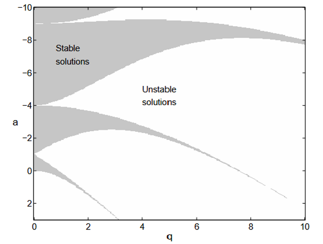
The classical equations of motion of a particle in a trap can be decoupled in each of x, y, and z. Let’s just look at x here.
\[\ddot{x} = -\frac{Z|e|}{m}\frac{\partial \Phi}{\partial x} = -\frac{Z|e|}{m}\left[U\alpha + \tilde{U}\cos(\omega_{\mathrm{rf}}t)\alpha'\right]x\]We can rearrange this to the standard form of the Mathieu differential equation:
\[\frac{d^2 x}{d\xi^2} + [a_x - 2q_x \cos(2\xi)]x = 0\] \[\xi = \frac{\omega_{\mathrm{rf}} t}{2}, \quad a_x = \frac{4Z|e|U\alpha}{m\omega_{\mathrm{rf}}^2}, \quad q_x = \frac{2Z|e|U\alpha'}{m\omega_{\mathrm{rf}}^2}\]
Z = number of elementary charges (almost always 1)
|e| = magnitude of the elementary charge (always \(1.602 x 10^{-19}\))
m = mass of ion
Check out the worked derivations page for the Mathieu equation for more details.
A trap is only stable if it falls into this stability diagram. If the q and a factors fall in the unstable region, then the ion will not stay trapped for long, if at all.
Pseudopotential, secular motion and micromotion
I said earlier that we can imagine this as a kid on a swing, and that is still true. The pseudopotential for a trapped ion can be approximated as \[\Phi_{\mathrm{pseudo}}(x) = \frac{1}{2}m\omega_{\mathrm{sec}}^2 x^2\]
The secular motion \(\omega_{sec}\) is the frequency of the swinging. It is typically low in speed but fairly high.
There is also another type of motion - the micromotion. This is the small jittering of the ion - far faster than the secular motion, but far smaller.
The psuedopotential for an ion in a trap is a harmonic oscillator operating at the secular frequency \[\Phi_{\mathrm{pseudo}}(x) = \frac{1}{2}m\omega_{\mathrm{sec}}^2 x^2\] with \[\omega_{sec} = \frac{\beta_x \omega_{rf}}{2} and \beta_x \approx \sqrt{a_x + \frac{q_x^2}{2}}\]
The lowest order approximation for the motion of a trapped ion is: \[x(t) = A\cos(\omega_{\mathrm{sec}}t)\left(1-\frac{q_x}{2}\cos(\omega_{\mathrm{rf}}t)\right)\]
The motion consists of harmonic oscillations at \(\nu = \beta_x \frac{\omega_{\mathrm{rf}}}{2} \ll \omega_{\mathrm{rf}}\). This is the secular motion, with micro motion at \(\omega_{rf}\). This micromotion is 180 degrees out of phase with the RF drive and is \(q_{x}/2\) smaller than the secular motion.
Modes of equally spaced ions in a linear chain
We have gone over the simple case - just one ion in a trap and just one direction. But the ion is moving all three directions, and when more ions get added it gets more complicated. All ions are charged, and they push on each other too.
We call the ways the ion moves the “modes of motion”. It moves in the direction of the trap - the axial direction. But also the other directions too - the radial directions. These modes move in patterns.
Take a look at the motional mode physics demo for a good look at it.
The ions will move in different modes of motion in the axial and radial directions. With more ions in the trap, we must consider the Coulomb repulsion of each ion on each other. The Coulomb stiffness is: \[C = \frac{e^2}{4\pi\epsilon_0 d^3}\]
We find these modes by finding the Hessian matrix. This is the second derivitive of the potential V.
In the axial direction: \[A_{ij} = \frac{\partial^2 V}{\partial z_i \partial z_j} = -\frac{2C}{|i-j|^3} \quad (i \neq j)\] \[A_{ii} = \kappa_i + \sum_{k \neq i} \frac{2C}{|i-k|^3}\]
In the radial direction \[B_{ij} = +\frac{C}{|i-j|^3} \quad (i \neq j)\] \[B_{ii} = m\omega_x^2 - \sum_{k \neq i} \frac{C}{|i-k|^3}\]
The eigenmodes of this matrix are the motional modes, and the eigenfrequencies are the mode frequencies.
\[A\vec{b}_m = m\omega_m^2\vec{b}_m\] \[B\vec{b}_m = m\omega_m^2\vec{b}_m\]
***Quantum motion
Since this is quantum computing after all, we can give these equations of motion the quantum mechanical treatment. We replace coordinates with operators.
Let’s write down the Hamiltonian of the motion. It is just the familiar static potential harmonic oscillator: \[\hat{H}^{(m)} = \frac{\hat{p}^2}{2m} + \frac{m}{2}W(t)\hat{x}^2\]
We can now write down the equations of motion of these p and x operators quantum mechanically too:
\[\dot{\hat{x}} = \frac{1}{i\hbar}[\hat{x},\hat{H}^{(m)}] = \frac{\hat{p}}{m}\] \[\dot{\hat{p}} = \frac{1}{i\hbar}[\hat{p},\hat{H}^{(m)}] = -mW(t)\hat{x}\]
We want to give these equations the quantum mechanical treatment.
We replace the x coordinate by the operator \(\hat{x}\), and we can write the potential as: \[V(t) = \frac{m}{2}W(t)x^2\] with \[W(t) = \frac{\omega_{\mathrm{rf}}^2}{4} \left[a_x + 2q_x\cos(\omega_{\mathrm{rf}}t)\right]\]
We can write the Hamiltonian of the motion as the static potential harmonic oscialltor: \[\hat{H}^{(m)} = \frac{\hat{p}^2}{2m} + \frac{m}{2}W(t)\hat{x}^2\]
Now we can write down the equations of motion in the Heisenberg picture:
\[\dot{\hat{x}} = \frac{1}{i\hbar}[\hat{x},\hat{H}^{(m)}] = \frac{\hat{p}}{m}\] \[\dot{\hat{p}} = \frac{1}{i\hbar}[\hat{p},\hat{H}^{(m)}] = -mW(t)\hat{x}\]
If we say that the solution to the Mathieu equation is u(t), then we can rewrite these quantum operators using a classical solution (this will be helpful later):
\[\hat{x}(t) = \sqrt{\frac{\hbar}{2m\nu}} \left[\hat{a}\,u^*(t) + \hat{a}^\dagger u(t)\right]\] \[\hat{p}(t) = \sqrt{\frac{\hbar m}{2\nu}} \left[\hat{a}\,\dot{u}^*(t) + \hat{a}^\dagger \dot{u}(t)\right]\]
Choosing the secular frequency
The secular frequency affects the computation a lot. Higher secular frequency means the ions are more tightly confined, but you will get a lower coupling to the motion.
Higher secular frequency:
-
Slower gates
-
Lower heating rates
-
Smaller Lamb-Dicke parameter
Quantum gates depend on the motion, detuning, and pulse duration. Higher secular frequency means a larger energy gap between elevels, and lower coupling strength - therefore slower gates. This can be compensated for with extra laser power.
Higher secular frequency means better ion confinement. This reduces the heating rates of the ions too. \[\dot{n} \propto \frac{S_E (\omega_{sec})}{\omega_{sec}}\] with \(S_e\) being the electric field noise spectral density.
Higher secular frequency also means a smaller Lamb-Dicke parameter. \[\eta = k_{x_0}\sqrt{\frac{\hbar}{2m\omega_{\mathrm{sec}}}}\]
***Planar trap scaling: depth, frequency and heating vs ion height
Placeholder
Placeholder
Lamb-Dicke regime and sidebands
The Lamb-Dicke Regime is when the ion’s wavefuntion is much less than the wavelength of the laser you are using.
When we are deep in the Lamb-Dicke Regime, all of our calcuations bcome easier.
The Lamb-Dicke Parameter is: \[\Eta = k*\sqrt{\frac{\hbar}{2m\nu}}\]
We can say we are operating in the Lamb-Dicke Regime when \(\Eta\) is much less than 1. Equivilently, when the ion’s wave function ins much less than the wavelength of the lasers we are using.
When we are in the Lamb-Dicke Regime, only the carrier and first order sidebands are relevant.
Equivilently: \[\Eta = k*x_0\] \[\Eta \sqrt{2\langle n \rangle + 1} \ll 1\]
Resolved vs unresolved sidebands
Think about rungs on a ladder. If we hit the center rung, that is what we aimed for.
If we drive a laser at the transition frequency, the center rung, then say we drive the “carrier”.
If we are off by the secular frequency, then we hit a rung one away than what we aimed for, then we drive a “sideband”.
The transition gives or creates one quanta motion, so the motion becomes a little hotter or colder, and the transition happens.
When the rungs are clear and we can hit the one we want, they are called “resolved sidebands”.
If the linewidth of the transition is larger than the motional frequency, then we can not hit the rung we want. We may aim for one and hit another. This is called “unresolved sidebands”. This is almost always bad.
The carrier frequency is the frequency of an optical transition that is being driven.
IF the frequency is exactly separated from the transition by the secular motion frequency, then the motion can give or take one quanta of motion to drive the transition. This is called a sideband.
\[\begin{array}{c|c} \text{Carrier} & |g,n\rangle \leftrightarrow |e,n\rangle \\ \text{RSB} & |g,n\rangle \leftrightarrow |e,n-1\rangle \\ \text{BSB} & |g,n\rangle \leftrightarrow |e,n+1\rangle \end{array}\]When the natural linewidth of a transition is much smaller than the motional frequency \[(\Gamma \ll \nu)\], then individual sidebands can not be spectrally resolved. These are called unresolved sidebands.
Resolved sidebands behave like the Janes-Cummings model.
Photoionization loading
When an atom goes to a new state, a new energy level, this is the electron being pushed farther away from the nucleus. If we push it far enough then the electron will fly off. An atom minus one electron is an ion.
Photoionization is a bound free electric dipole transition.
If a bound electron in state \(|nl\rangle\) absorbs a photon of energy \(\hbar\omega\) and \(\hbar\omega > E_I\) then the final state is a continuum state. An electron leaving the atom and moving in the atom’s Coulomb field.
Autoionization is when the atom first goes to a discrete state whose energy is above the ionization limit, and the internal electron-electron interaction throws one electron out. Photoionization just pushes the electron past the ionization threshold and to the continuum. But autoionization pushies it to a discrete state past the continuum, then it gets thrown out.
Fermi’s Golden Rule gives the rate. The transition rate between quantum states caused by a weak perturbation is:
\[\Gamma_{i\rightarrow f} =\frac{2\pi}{\hbar} \left|\langle f|\hat{V}|i\rangle\right|^2 \rho(E_f)\]The perturbation here is the interaction between electron and laser. This gives the rate as:
\[\Gamma =\frac{2\pi}{\hbar}\frac{e^2 E_0^2}{4}|r_{fi}|^2\]Where \(r_{fi} =\langle E,f|\hat{\boldsymbol{\epsilon}}\cdot\mathbf r|i\rangle\). This matrix element describes how strongly the laser couples the initial state to the final continuum state. (This is normalized to make it easier - this removes the density of states)
***Heating rates and motional decoherence
Placeholder
Placeholder
Cooling
Doppler cooling
When you think of lasers you think of Superman’s heat vision or laser blasts in Star Wars. You think lasers heat things up. But here, we are going to use lasers to cool things down.
Imagine a kid on a swing. You have to slow them down, but you can only push. What do you do?
You push when they are coming toward you, and do nothing when they are going away from you.
This is the whole idea behind Doppler cooling. We take advantage of the doppler effect to do this.
Have you ever heard a motorcycle on the road? It sounds different coming towards you than away from you. The frequency of the sound seems higher when it comes toward you, and lower when it goes away from you. We can exploit this.
Atoms can absorb certain colors (frequencies) of light. We can tune the frequency of the laser just a little below this line. When the atom moves away from us the Doppler effect takes part and makes us look even farther off of the right frequency. But when the atom comes towards us the frequency looks perfect and the atom absorbs the light, spits it back out, and loses a little speed. We repeat this over and over again until the atom is very very slow.
A slow atom happens to be the definition of cold. Therefore we have cooled the atom. This is called “Doppler Cooling”.
If you red detune a laser that drives the transition between an atoms ground and excited states, the atom is only resonant with the transition when it moves one direction (Doppler Effect).
The ion will absorb the photon in one direction and cool, and emit the photon in a random direction and heat. The ion will slow down in the same direction over and over again, and heat a small amount in a random direction.
Using this strategy we can cool the atom to near absolute zero. Because this cooling method depends on absorbtion, we can never cool it to the ground state. It is a balance of heating and cooling. The Doppler limit is \[K_B T_D = \frac{\hbar \Gamma}{2}\] with \(\Gamma\) being the linewidth of the transition. \[\bar{n}=\frac{\Gamma}{2\nu} \gg 1\]
Resolved-sideband cooling
Remember those sidebands from earlier:
\[\begin{array}{c|c} \text{Carrier} & |g,n\rangle \leftrightarrow |e,n\rangle \\ \text{RSB} & |g,n\rangle \leftrightarrow |e,n-1\rangle \\ \text{BSB} & |g,n\rangle \leftrightarrow |e,n+1\rangle \end{array}\]We can use the red sideband (laser off from a transition by the secular frequency) to remove one phonon of motion and cool one single mode of motion down. The ion will decay back to the ground state, and the speed is gone. Repeat this over and over again until there are no phonons left.
Keep in mind we are cooling the mode of motion, not the ion. So if ther are many ions in a chain, they all cool in that direction at once, but we have to repeat for other modes. More ions means more modes means more cooling we have to do.
The prerequisites of Resolved Sideband cooling are:
-
Must be in the Lamb-Dicke Regime \((n\sqrt{\bar{n}}) \ll 1\)
-
Must have resolved sidebands \((\nu \gg \Gamma)\)
We can use a narrow linewidth laser on a Red Sideband \((|g,n\rangle \leftrightarrow |e,n-1\rangle)\) detuned by the secular frequency of one mode. The ion will absorb the photon, and transition to the excited state while losing one phonon in that mode. The ion will decay back to the ground state but the phonon will stay removed. This can be done enough times so the odds that it is cooled to the ground state is near 100%. Since we can not be 100% sure that all phonons are removed, we say that the final phonon number is \(\bar(n) \ll 1\).
The average final phonon number is: \[\bar{n}_{min} = \frac{\gamma^2}{4\nu^2 + \gamma^2} \ll 1\]
EIT cooling
EIT cooling stands for Electromagnetically Induced Transparency cooling/ This is another type of laser cooling.
This strategy uses a probe beam and a control beam. These two beams destructively interfere with each other, and creates a “dark resonance”. The carrier is completely dark - the ion can not see that light. The red sideband absorbtion is very high, and the blue sideband is very low.
Many modes see this effect. So many modes absorb the RSB a lot, the carrier 0, and the BSB just a little. IT can not get the modes to the ground state, but it gets many modes below the Doppler limit fast. Faster, but not quite as good as Sideband Cooling.
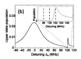
EIT Cooling is a way to engineer the absorption spectrum so that the red sideband transitons are favored over the carrier and blue sidebands.
Requirements:
-
A three level Lambda system
-
Resolved sidebands \((\nu \gg \Gamma)\)
Two lasers (the probe beam and control beam) couple different ground states to the same excited state.
\[|g_1\rangle \leftrightarrow |e\rangle\] \[|g_2\rangle \leftrightarrow |e\rangle\]
These two excitation pathways interfere, therefore it creates a superposition - the “dark state”
\[|D\rangle = \frac{\Omega_2 |g_1\rangle - \Omega_1 |g_2\rangle}{\sqrt{|\Omega_1|^2 + |\Omega_2|^2}}\]The interaction Hamiltonian can be written as:
\[H_I = \frac{\hbar}{2}\left(\Omega_p |e\rangle\langle g_1| + \Omega_c |e\rangle\langle g_2|\right) + \mathrm{h.c.}\] \[H_I |D\rangle = \frac{\hbar}{2\sqrt{\Omega_c^2 + \Omega_p^2}} \left(\Omega_p\Omega_c - \Omega_c\Omega_p\right)|e\rangle = 0\] \[H_I |D\rangle \propto \Omega_p\Omega_c - \Omega_c\Omega_p = 0\]The two excitation amplitudes cancel - therefore the dark stat is not coupled to the excited state by the laser interaction.
Similarly, this can be done for the RSB and BSB to show that RSB has high absorbtion coupling and the BSB has low.
This interaction creates a broad range of frequencies where RSB absorption is stronger than BSB absorption, therefore in works for multiple modes at once.
If we define A- as the phonon removal rate of the RSB, and A+ as the phonon addition rate of the BSB, then we can find the average final phonon number as:
\[\bar{n}_m = \frac{A_+(\omega_m)}{A_-(\omega_m) - A_+(\omega_m)}\]
Building the full Hamiltonian
Qubit Hamiltonian
The qubit Hamiltonian is:
\[H = \frac{\hbar \omega _0}{2} \sigma _z\]The ground and excited electronic states have different energies:
\[E_e = +\frac{\hbar \omega _0}{2}\] \[E_g = -\frac{\hbar \omega _0}{2}\]Therefore the energy separation is
\[\Delta E = E_e - E_g = \hbar \omega _0\]Trap/Motion Hamiltonian
The Hamiltonian of the trap/motion is:
\[H_motion = \frac{p^2}{2m} + \frac{1}{2} M \omega _z ^2 x^2\]This is just an ion in a harmonic oscillator. The first term is kinetic energy. The second term is potential energy.
This can be quantized as:
\[H_motion = \hbar \omega _z (a^{\dagger}a + \frac{1}{2})\]The Hamiltonian of the trap/motion is:
\[H_motion = \frac{p^2}{2m} + \frac{1}{2} M \omega _z ^2 x^2\]This is just an ion in a harmonic oscillator. The first term is kinetic energy. The second term is potential energy.
Now we can introduce the creation and nannihilation operators:
\[a = \sqrt{\frac{m\omega_z}{2\hbar}} \left( \hat{x} + \frac{i\hat{p}}{m\omega_z} \right)\] \[a^\dagger = \sqrt{\frac{m\omega_z}{2\hbar}} \left( \hat{x} - \frac{i\hat{p}}{m\omega_z} \right)\]Similarly, the momentum operator is:
\[\hat{p} = -im\omega_z x_0 (a - a^\dagger)\]We can sub these in, and use the identity \([a,a^\dagger] = 1\) to get:
\[H_motion = \hbar \omega _z (a^{\dagger}a + \frac{1}{2})\]What does this tell us? We use this with the number operator \(\hat{n}=a^\dagger a\) which satisfies \(a^\dagger a |n\rangle = n|n\rangle\). Therefore:
\[H_{motion}|n\rangle = \hbar \omega _z (n+\frac{1}{2})|n\rangle\]The possible motional energies are:
\[E_n = \hbar \omega _z(n+\frac{1}{2})\]Laser\Ion Interaction Hamiltonian
Subbing in \(\hat{x}\) and moving to the interaction picture (using RWA) gives:
\[H_I = \frac{\hbar \Omega}{2}(\sigma_+ e^{i \Eta_m (a_m + a_m^{\dagger})} e^{-i\delta t} e^{i\phi} + h.c.)\]Rearrange to get:
\[H_I = \frac{\hbar \Omega}{2}(\sigma_+ e^{i(k\hat{x} - \omega_L t _ \phi)} + h.c.)\]Subbing in \(\hat{x}\) and moving to the interaction picture (using RWA for a single relevent mode m) gives:
\[H_I = \frac{\hbar \Omega}{2}(\sigma_+ e^{i \Eta_m (a_m + a_m^{\dagger})} e^{-i\delta t} e^{i\phi} + h.c.)\]System Bath Coupling
The free evolving Hamiltonian of a system coupled to a bath is:
\[H_{B/C} = \Sigma _i \frac{\kappa _i}{2} \otimes (b_i + b_i^\dagger) \]-
\(\kappa\) is the coupling strength
-
\(\sigma _z\) is the qubit
-
\((b_i + b_i^\dagger)\) is the bath mode
The free evolving Hamiltonian of a system coupled to a bath is:
\[H_{B/C} = \Sigma _i \frac{\kappa _i}{2} \otimes (b_i + b_i^\dagger) \]-
\(\kappa\) is the coupling strength
-
\(\sigma _z\) is the qubit
-
\((b_i + b_i^\dagger)\) is the bath mode
If only \(\sigma _z\) is there, then that means there is only dephasing. There is no population transfer happening here. The system and the bath are just mixing and evolving.
Free evolving Hamiltonian (of bath)
The free evolving Hamiltonian is:
\[H_B = \Sigma _i \nu _i b_i^\dagger b_i\]The free evolving Hamiltonian is:
\[H_B = \Sigma _i \nu _i b_i^\dagger b_i\]This is just a collection of independent harmonic oscilators. This is just how the bath evolves in time.
In the interaction picture this becomes:
\[b_i(t) = b_i(0) e^{-i\nu _i t}\]Schrödinger Picture
This is a way to view or formulate Quantum Mechanics.
In the Schrödinger Picture:
-
States evolve in time
-
Operators are fixed
Imagine a movie. The camera is fixed, but the actors move around the camera.
In the Schrödinger Picture:
-
States evolve in time
-
Operators are fixed
The Schrödinger equation is:
\[i\hbar\frac{\partial}{\partial t}|\Psi(t)\rangle = \hat{H}|\Psi(t)\rangle\]The Hamiltonian doesn’t depend on time, so:
\[|\Psi(t)\rangle = e^{-\frac{i}{\hbar}\hat{H}t}|\Psi(0)\rangle\]with U(t) as the time evoltuion operator
\[U(t) = e^{-\frac{i}{\hbar}\hat{H}t}\]The expectation value of an observable is the same as the Heisenberg Picture:
\[\langle \hat{A} \rangle = \langle \Psi(t)|\hat{A}|\Psi(t)\rangle\]Example: Free Particle \((\hat{H} = \frac{\hat{p}^2}{2m})\)
Starts in Gaussian wavepacket at t=0:
\[\Psi(x,0) = \frac{1}{\sqrt{2\pi\sigma}}e^{-\frac{x^2}{4\sigma^2}}e^{\frac{ip_0x}{\hbar}}\]State’s shape spreads in time - the wavepacket evolves.
Heisenberg Picture
In the Heisenberg Picture
-
States are fixed
-
Operators evolve in time
Imagine a movie. But the camera is strapped to the actors head. Like it is in first person. The actors look still, but the world moves around them.
In the Heisenberg Picture
-
States are fixed
-
Operators evolve in time
The operator is: \[\hat{A}_H(t) = e^{\frac{i}{\hbar}\hat{H}t}\hat{A}_S e^{-\frac{i}{\hbar}\hat{H}t}\]
with \(A_s\) being the operator in the Schrodinger Picture. The exponential moves the time depencence from the state to the operators.
The Schrodinger equation is not time dependent:
\[|\Psi_H(t)\rangle = |\Psi_S(0)\rangle\]The equation of motion is:
\[\frac{d\hat{A}_H}{dt} = \frac{i}{\hbar}[\hat{H},\hat{A}_H] + \left(\frac{\partial\hat{A}_S}{\partial t}\right)_H\]The \(\frac{i}{\hbar}[\hat{H},\hat{A}_H]\) shows how the observable evolves.
The \(\left(\frac{\partial\hat{A}_S}{\partial t}\right)_H\) is the average time dependence - an external field or somthing.
Example: Free Particle (\(\hat{H} = \frac{\hat{p}^2}{2m}\))
Momentum (no force on free particle):
\[\frac{d\hat{p}_H}{dt} = \frac{i}{\hbar}[\hat{H},\hat{p}_H] = 0\]Position (position changes with time):
\[\frac{d\hat{x}_H}{dt} = \frac{i}{\hbar}[\hat{H},\hat{x}_H] = \frac{\hat{p}_H}{m}\]Expectation of Observables:
\[\langle\hat{A}\rangle = \langle\Psi_H|\hat{A}_H(t)|\Psi_H\rangle\]Interaction Picture
In the Interaction Picutre:
-
Both states and operators evolbe in time
-
Evolution due to \(\hat{H}_0\) is to the operators
-
Evolution due to \(\hat{V}\) is to the states
In the Interaction Picutre:
-
Both states and operators evolbe in time
-
Evolution due to \(\hat{H}_0\) is to the operators
-
Evolution due to \(\hat{V}\) is to the states
How operators evolve (equation of motion):
\[\hat{A}_I(t) = e^{\frac{i}{\hbar}\hat{H}_0 t}\hat{A}_S e^{-\frac{i}{\hbar}\hat{H}_0 t}\]How states evolve:
\[\hat{V}_I(t) = e^{\frac{i}{\hbar}\hat{H}_0 t}\hat{V}_S e^{-\frac{i}{\hbar}\hat{H}_0 t}\]Same Schrodinger equation as Schrodinger Picture, but simpler:
\[i\hbar\frac{\partial}{\partial t}|\Psi_I(t)\rangle= \hat{V}_I(t)|\Psi_I(t)\rangle\]Example: driven two-level atom
To get the total Hamiltonian all you need is the standard atom Hamiltonian and then add the laser interaction Hamiltonian.
\[\hat{H} = \hat{H}_0 + \hat{V}_I\] \[\hat{H}_0 = \frac{\hbar \omega _0}{2} \hat{\sigma}_z\] \[\hat{V}_I = \frac{\hbar \Omega}{2}[e^{i \Delta t} \hat{\sigma}_+ + e^{-i \Delta t} \hat{\sigma}_-]\]We know the standard two level atom Hamiltonian is:
\[\hat{H}_0 = \frac{\hbar \omega _0}{2} \hat{\sigma}_z\]We know the laser interaction Hamiltonain is:
\[\hat{V}_s (t) = -\hat{d} \times E(t)\] \[\hat{d} = d_{ge} \hat{\sigma}_+ + d_{eg} \hat{\sigma}_-\] \[E(t) = E_0 cos(\omega t)\] \[\hat{V}_s (t) = \hbar \Omega cos(\omega t) (\hat{\sigma}_+ + \hat{\sigma}_-)\]We must take this interaction Hamiltonian and go to the interaction picture \([A_I(t) = U_0^{\dagger} \hat{A}_s U_0(t)]\):
\[\sigma_{\pm} = e^{\pm i \omega _0 t} \hat{\sigma}_{\pm}\] \[\sigma_z (t) = \sigma_z\] \[V_I(t) = U_0^{\dagger} \hat{V}_s U_0(t)\] \[V_I(t) = \hbar \Omega cos(\omega t) [e^{i\omega _0 t}\sigma _+ + e^{-i\omega _0 t}\sigma _-]\] \[cos(\omega t) = \frac{1}{2}[e^{i\omega t} + e^{-i \omega t}]\] \[V_I(t) = \frac{\hbar \Omega}{2} [e^{i(\omega _0 + \omega)t}\sigma _+ + e^{-i(\omega _0 - \omega)t}\sigma _+ + e^{-i(\omega _0 + \omega)t}\sigma _- + e^{i(\omega _0 - \omega)t}\sigma _-]\]Now we can set \(\Delta = \omega + \omega _0\) and use the Rotating Wave Approximation to remove the fast rotating terms. This simplifies the equation greatly.
\[V_I(t)^{RWA} = \frac{\hbar \Omega}{2} [e^{i\Delta t}\sigma _+ + e^{-i\Delta t}\sigma _- ]\]This is the completed Hamiltonian for the laser interaction. Now we just add in the original two level atom Hamiltonian and we are done.
\[\hat{H} = \hat{H}_0 + \hat{V}_I\] \[\hat{H} = [\frac{\hbar \omega _0}{2} \hat{\sigma}_z] + [\frac{\hbar \Omega}{2}[e^{i \Delta t} \hat{\sigma}_+ + e^{-i \Delta t} \hat{\sigma}_-]]\]Example: three-level S–P–D system (Ba⁺)
We have the basic Hamiltonian of a 3 level system:
\[H_0 = E_S |S\rangle \langle S| + E_P |P\rangle \langle P| + E_D |D\rangle \langle D|\]Plus the laser interaction Hamiltonian:
\[H_L = \Sigma_{i=S,D} \hbar \Omega_i cos(\omega_i t)(|i\rangle \langle p| + h.c.)\]Which gives:
\[H_I = \hbar \Delta_S |S\rangle \langle S| + \hbar \Delta_D |D\rangle \langle D| + \frac{\hbar \Omega_S}{2}(|S\rangle \langle P| + |P\rangle \langle S|) + \frac{\hbar \Omega_D}{2}(|D\rangle \langle P| + |P\rangle \langle D|)\]Let’s take Ba 138+ as an example.
\[H_0 = E_S |S\rangle \langle S| + E_P |P\rangle \langle P| + E_D |D\rangle \langle D|\]Laser frequencies: \(\omega_S = \omega_{0,S} + \Delta_S\), \(\omega_{0,S} = \frac{E_P-E_S}{\hbar}\) \(\omega_D = \omega_{0,D} + \Delta_D\), \(\omega_{0,D} = \frac{E_P-E_D}{\hbar}\)
The laser interaction Hamiltonian is:
\[H_L = \Sigma_{i=S,D} \hbar \Omega_i cos(\omega_i t)(|i\rangle \langle p| + h.c.)\] \[H_I = e^{\frac{iH_0^' t}{\hbar}}(H-H_0^')e^{\frac{-iH_0^' t}{\hbar}} = \hbar \Delta_S |S\rangle \langle S| + \hbar \Delta_D |D\rangle \langle D| + e^{\frac{iH_0^' t}{\hbar}}(H_L)e^{\frac{-iH_0^' t}{\hbar}} + h.c.\] \[e^{\frac{iH_0^' t}{\hbar}}(H_L)e^{\frac{-iH_0^' t}{\hbar}} = \Sigma_k \hbar \Omega_k cos(\omega_k t)e^{\frac{iH_0^' t}{\hbar}} |k\rangle \langle p| e^{\frac{-iH_0^' t}{\hbar}} + h.c.\]Let \(\Delta_P = 0, k= S,P,D\). -> \(e^{\frac{iH_0^' t} = \Sigma_k e^{i(E_k-\Delta_k \hbar) \frac{t}{\hbar}}|k\rangle \langle k|\) and \(cos(\omega t) = \frac{1}{2}(e^{i\omega t} + e^{-i\omega t})\)
\[e^{\frac{iH_0^' t}{\hbar}}(H_L)e^{\frac{-iH_0^' t}{\hbar}} = \Sigma_k \frac{\hbar \Omega_k}{2}(e^{i\omega t} + e^{-i\omega t})e^{i(E_k-\Delta_k \hbar) \frac{t}{\hbar}}|k\rangle \langle P| e^{iE_P\frac{t}{\hbar}}\]Simplify using RWA:
\[H_I = \Sigma_k \frac{\hbar \Omega_k}{2}(1+e^{-i2\omega_k t})|k\rangle \langle P| + h.c. \] \[H_I = \hbar \Delta_S |S\rangle \langle S| + \hbar \Delta_D |D\rangle \langle D| + \frac{\hbar \Omega_S}{2}(|S\rangle \langle P| + |P\rangle \langle S|) + \frac{\hbar \Omega_D}{2}(|D\rangle \langle P| + |P\rangle \langle D|)\]***Dipole interaction
An atom has a positive nucleus (protons and neutrons) and negative electrons. These can be displaced causing an “electric dipole moment”.
Placeholder
***Electric-dipole selection rules
Placeholder
Placeholder
The trapped-ion Hamiltonian, piece by piece
Qubit Hamiltonian:
\[H = \frac{\hbar \omega _0}{2} \sigma _z\] \[\sigma _z = |e\rangle \langle e| - |g\rangle \langle g|\]Trap/Motion Hamiltonian:
\[H_{motion} = \frac{p^2}{2m} + \frac{1}{2} M \omega _z ^2 x^2\]This can be quantized as:
\[H_motion = \hbar \omega _z (a^{\dagger}a + \frac{1}{2})\]Laser interaction Hamiltonian:
\[\hat{V}_s (t) = -\hat{d} \times E(t)\] \[H_I = H_0 + V_s = \frac{\hbar \Omega}{2}(\sigma_+ e^{i(k\hat{x} - \omega_L t _ \phi)} + h.c.)\]Coupling to bath:
\[H_{B/C} = \Sigma _i \frac{\kappa _i}{2} \otimes (b_i + b_i^\dagger) \]Free evolving Hamiltonian (of bath):
\[H_B = \Sigma _i \nu _i b_i^\dagger b_i\]Qubit Hamiltonian:
\[H = \frac{\hbar \omega _0}{2} \sigma _z\] \[\sigma _z = |e\rangle \langle e| - |g\rangle \langle g|\]Trap/Motion Hamiltonian:
\[H_motion = \frac{p^2}{2m} + \frac{1}{2} M \omega _z ^2 x^2\]This can be quantized as:
\[H_motion = \hbar \omega _z (a^{\dagger}a + \frac{1}{2})\]Laser interaction Hamiltonian:
\[\hat{V}_s (t) = -\hat{d} \times E(t)\] \[\hat{d} = d_{ge} \hat{\sigma}_+ + d_{eg} \hat{\sigma}_-\] \[E(t) = E_0 cos(\omega t)\] \[\hat{V}_s (t) = \hbar \Omega cos(\omega t) (\hat{\sigma}_+ + \hat{\sigma}_-)\] \[H_I = H_0 + V_s = \frac{\hbar \Omega}{2}(\sigma_+ e^{i(k\hat{x} - \omega_L t _ \phi)} + h.c.)\]Coupling to bath:
\[H_{B/C} = \Sigma _i \frac{\kappa _i}{2} \otimes (b_i + b_i^\dagger) \]Free evolving Hamiltonian (of bath):
\[H_B = \Sigma _i \nu _i b_i^\dagger b_i\]Gate Evolution Operator for Two Qubit Entangling Gate
The gate evolution unitary is:
\[\hat{U}(t) = \exp\left[\sum_{j=1}^{2}\left(\alpha_j(t)a^\dagger - \alpha_j^*(t)a\right)\hat{\sigma _z^j - i\frac{\theta}{2}(t)\hat{\sigma}_z^1\hat{\sigma}_z^2\right]\]The gate evolution unitary is:
\[\hat{U}(t) = \exp\left[\sum_{j=1}^{2}\left(\alpha_j(t)a^\dagger - \alpha_j^*(t)a\right)\hat{\sigma _z^j - i\frac{\theta}{2}(t)\hat{\sigma}_z^1\hat{\sigma}_z^2\right]\]Raman gates
Introduction
Imagine you are standing on top of a bus going 100 mph. If you throw a baseball backwards at 90 mph - then to someone standing on the side of the road the baseball looks like it is moving 10 mph. That is similar to the idea behind a Raman transition.
If we need a laser frequency far smaller than the lasers we have, then we can try a Raman transition.
I’ss use easy numbers here for this example. Say we have an atom with a 10 GHz splitting, but we have no 10 GHz laser. But we have one laser at 100 THz. And we have another laser at 100 THz + 10 GHz = 100.010 THz (or we can split our beam and tune one side up 10 GHz). If we poin both of those lasers at an atom, and one photon from each of those lasers hits the atom at the same time, then the atom will do what we call a “virtual transition”.
Similar to throwing a baseball on a moving bus, the atom will see the 10 GHz frequency difference and the transition will occur.
The lasers must be far away from any other transtions for this to work, and there are a few other requirements too, but that is the general idea of a Raman transition.
A Raman transition is a two photon transition. It is also called a “virtual transition”.
These two photons are detuned from each other by the same frequency of an atomic transition. One photon virtually excites the atom. The second photon decays the atom down from the virtually excited state and into the nearby atomic state whose transition frequency is equal to the difference in frequency of the two photons used in the virtual transition.
The k vector of the lasers must have some component along the quantization axis.
Using this method we can do X, Y, and Z rotations between the two nearby states by tuning the phases of the lasers and frequency detuning.
The ¹³⁷Ba⁺ qubit
The hyperfine splitting of Ba137+ splits the ground state into different sublevels. This is the \(S\frac{1}{2}\) level. A Raman transition is typically done to do a swap between these ground states. The splitting between these \(S\frac{1}{2}\) sublevels is 8.037 GHz.
A Raman transition is typically done on the \(S\frac{1}{2}\) sublevels.
\[|0\rangle = |S\frac{1}{2}, F=1, m_F=0\] \[|1\rangle = |S\frac{1}{2}, F=2, m_F=0\] \[\frac{\omega _{HF}}{2 \pi} = 8.037 GHz\]Since we are using the \(m_F=0\) sublevels we say that this transition is magnetic field insensitive to the first order.
The Raman transition and the polarization rule
A Raman transition can only happen if the combined laser polarizations of the laser point in the direction of the magnetic field even a little bit.
The two raman beams have polarizations \(\hat{\varepsilon _1}\) and \(\hat{\varepsilon _2}\).
The laser polarization requirement for driving a Raman transition is:
\[(\hat{\varepsilon _1} \times \hat{\varepsilon _2} \dot \rightarrow{B} \neq 0)\]i.e. the tensor product of the two laser polarizations need to have some component along the B field.
Raman gate Hamiltonian and single-qubit rotations
Adjusting the phase difference between the two lasers will determine your rotation axis.
Adjusting your laser intensity is your rotation speed.
Adjusting the tume of the pulse is the amount of rotation.
The Raman transition Hamiltonian is:
\[H = \frac{\hbar \Omega _{eff}}{2} [e^{i\phi} |1\rangle \langle 0| + e^{-i\phi} |0\rangle \langle |] + \frac{\hbar \delta}{2} \sigma _z\] \[H = \frac{1}{2} [\Omega _x X + \Omega _y Y] + \delta Z\] \[\phi = \phi _1 - \phi _2\] \[\Phi _{eff} = \Delta k \dot r = \delta t _ \phi\]-
\(\Delta k \dot r\) = Spatial Phase
-
\(\delta t\) = Frequency Difference
-
\(\phi\) = Optical Phase
For a pure X rotation:
-
\(\delta\) = 0
-
\(\phi\) = 0
-
\(\theta = \Omega _{eff} t = \pi\) - (For a Hadamard Gate \(\theta = \frac{\pi}{2}\))
For a pure Y rotation:
-
\(\delta\) = 0
- \(\phi = \frac{\pi}{2}\)
-
\(\theta = \Omega _{eff} t = \pi\)
For a pure Z rotation:
- \(\delta \neq -\)
-
You can do a Z rotation. But Z rotations are typically done in software by just redefining the phases of X and Y the software is tracking.
The k-vector
The k vector is the direction the laser is pointing. We care about the difference between each laser’s k vector.
\[k=\frac{2\pi}{\lambda} \hat{n}\] \[|\Delta k| = |k_1 - k_2| = 2k sin(\theta)\]The k vector is the direction the laser is pointing.
\[k=\frac{2\pi}{\lambda} \hat{n}\] \[|\Delta k| = |k_1 - k_2| = 2k sin(\theta)\]Co-propagating beams will have an angle of \(\theta = 0\) and therefore a k vector of \(\Delta k = 0\).
Counter propagating beams will have an angle of \(\theta = \pi\) and therefore a k vector of \(\Delta k = \frac{4\pi}{\lambda}\)
The effective Rabi rate depends on the k vector as well:
\[\Omega _x = \Omega _{eff} e^{i(\Delta kx - \Delta \omega t + \phi)}\]Two-qubit Mølmer-Sørensen gate: idea and steps
The whole idea for a 2 qubit gate is we want a different outcome if the qubits are in the state \(|11\rangle\) than if they are in any other state (up to a single qubit rotation).
One way to do this is throught the Molmer-Sorenson Gate. This gate works by moving the qubit in phase space (the space where position is on the x axis and momentum is on the y axis). When it travels in this phase space it accumulates phase based on the area that it moved. If we push the qubit in a circle and time it so we stop pushing when it ends up exactly where it started then the qubit looks the same, but gains this phase. The whole idea is that we want the \(|11\rangle\) state to gain a phase, while it cancels out for every other state (up to a single qubit rotation).
We do this by using both the red and blue sidebands. This makes a “bichromatic field” that pushes \(|0\rangle\) and \(|1\rangle\) in opposite directions.
Steps:
-
Choose a motional mode (like axial COM)
-
Apply both RSB and BSB on both ions. Motion is virtually excited.
-
Turn the beams off when ions return to starting position. The system will keep the aquired spin-dependent phase.
-
Result: Maximally entangled MS gate
MS Hamiltonian:
\[H = \hbar \Omega [\sigma_x^{(1)} + \sigma_x^{(2)}][ae^{-i\delta t} + a^{\dagger}e^{i\delta t}]\]-
\(|00\rangle\) -> \(e^{i\phi}|00\rangle\)
-
\(|01\rangle\) or \(|10\rangle\) -> \(|01\rangle\) or \(|10\rangle\)
-
\(|11\rangle\) -> \(e^{i\phi} |11\rangle\)
One Raman beam has 2 tones for RSB and BSB
-
RSB -> \(1,n\rangle \leftrightarrow |0,n+1\rangle\)
- \(\omega = \omega_{HF} - \omega_{motion} + \delta\)
-
BSB -> \(1,n\rangle \leftrightarrow |0,n-1\rangle\)
- \(\omega = \omega_{HF} + \omega_{motion} + \delta\)
The RSB and BSB make a bichromatic field. This forms a spin-dependent force that pushes \(|0\rangle\) and \(|1\rangle\) in opposite directions. We turn the beam off when the motion returns to 0, and the acquired geometric phase remains.
Steps:
-
Choose a motional mode (like axial COM)
-
Apply both RSB and BSB on both ions. Motion is virtually excited.
-
Turn the beams off when ions return to starting position. The system will keep the aquired spin-dependent phase.
-
Result: Maximally entangled MS gate
When the Hamiltonian is integrated over gate time:
\[U=e^{-i\phi}\sigma_x^{(1)}\sigma_x^{(2)}\]Phase-sensitive vs phase-insensitive gates
Quantum gates can be phase sensitive or phase insensitive. We want our gates to not depend on phase of the laser when it hits the ion. If the phase is a little off, or the path length fluctuates at nanometer scale (which happens often) we do not want this to cause a gate error.
There are ways we can tune our gates to avoid this.
Placeholder
Phase Sensitive 1Q Raman Gate
If both Raman beams hit the ion from opposite directions then the k vector is not 0. This means that the gate is phase sensitive
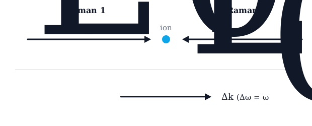
If both Raman beams hit the ion from opposite directions then the k vector is not 0. This means that the gate is phase sensitive.
The benefit here is that we can do phase sensitive single qubit gates with linearly polarized beams. This means we can get rid of the 4 photon Stark shift from a pulsed laser.
Phase In-Sensitive 1Q Raman Gate
If the beams are co-propagating then they travel the same path. This means the k vector is 0, and the gate is phase insensitive.
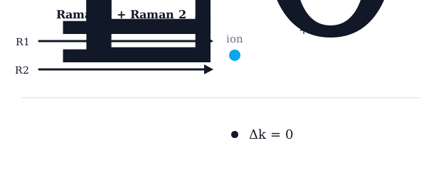
Because we do not have multiple tones when doing 1Q rotations, the only method we can make a 1Q gate phase insenstive is co-propagting the Raman beam such that \(\Delta k = k_1 - k_2 = 0\).
But remember, if the co-propagating beams have the same linear polarization then the outer product is 0, and there is not component along the magnetic field, so the transition can not occur.
So to do a phase insensitive 1Q Raman gate, we must use eliptically polarized beams. This means the 4 photon Stark shift from a pulsed laser will be present.
Phase Sensitive 2Q Raman Gate
Both the BSB and RSB frequency will be larger than the frequency of second beam we need to do the gate. Therefore \(\Delta k\) will always point right and will never be 0. Therefore, it is phase sensitive
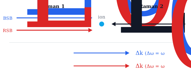
Because the qubit frequency \((\omega_0)\) is larger than the gate detuning \((\delta)\), the frequency of Raman 1 is always larger than the frequency of Raman 2. The effective wavevector will always point right, and any imbalanceb etween the two Raman paths will accululate to phase. Therefore it is phase sensitive.
Phase In-Sensitive 2Q Raman Gate
If we cleverly tune the tones of our Raman beam then we can make the BSB bigger than Raman 2 and RSB smaller than Raman 2.
This way the phases will cancel out, not accumulate. Therefore, it is phase insensitive.
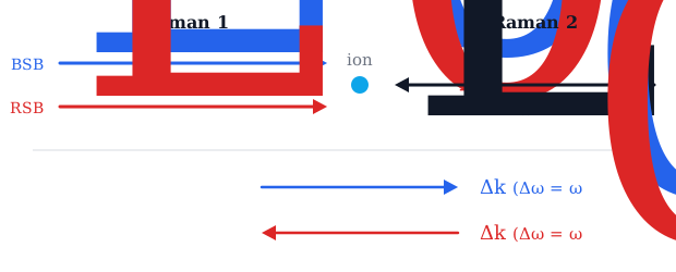
This time, we can cleverly tune the sidebands:
-
BSB = \(\omega_L + \omega_0 +\delta\) (standard)
-
RSB = \(\omega_L - \omega_0 + \delta\)
Now the k vectors are reversed. Raman 1 will be larger in the BSB case, and Raman 2 will be larger in the RSB case. The k vector will be in opposite directions and will cancel. Therefore, it is phase insensitive.
The only difference is how to apply tones on Raman beams
Two Qubit Gates
Introduction
A normal computer bit can be either 0 or 1.
A qubit can be in a state \(|0\rangle\), state \(|1\rangle\), or a superpositiob of both:
\[|\psi\rangle = \alpha|0\rangle + \beta|1\ranlge\]We can visualize a qubit as an arrow pointing somwehre on a sphere called the Bloch Sphere:
INSERT BLOCH SPHERE PICTURE
Every “gate” we talk about can be visualized as just a rotation on this sphere
A normal computer bit can be either 0 or 1.
A qubit can be in a state \(|0\rangle\), state \(|1\rangle\), or a superpositiob of both:
\[|\psi\rangle = \alpha|0\rangle + \beta|1\ranlge\]We can visualize a qubit as an arrow pointing somwehre on a sphere called the Bloch Sphere:
INSERT BLOCH SPHERE PICTURE
Every “gate” we talk about can be visualized as just a rotation on this sphere
CZ Gate
This is a 2 qubit gate. If the control qubit is 1 then the phase of the target qubit flips. If the control qubit is 0 then nothing happens.
-
\(|00\rangle\) -> \(|00\rangle\)
-
\(|01\rangle\) -> \(|01\rangle\)
-
\(|10\rangle\) -> \(|10\rangle\)
-
\(|11\rangle\) -> \(-|11\rangle\)
Implementation Steps:
-
RSB \(\pi\) pulse on ion 1. \(|1\rangle (n=0)\) -> \(|0\rangle (n=1)\). Else, nothing.
-
BSB \(2\pi\) pulse on ion 2. \(|1\rangle (n=1)\) to another state and back. This picks up a -1 phase only if both ions were in the \(|1\rangle\) state to start.
-
RSB \(\pi\) pulse on ion 1. This returns it to starting state.
The whole idea is we use sidebands to our advantage:
The RSB on ion 1 will do nothing to the \(|0\rangle\) state, but will change the \(|1\rangle\) state, and more importantly it creates a phonon in the mode.
The BSB \(2\pi\) pulse on ion 2 only works if there is a phonon in the mode (if the RSB last step worked) and only if it is in the \(|1\rangle\) state right now. This just pushes it to a new state and back - and more importantly pickes up a phase. Both ions have to have started in the \(|1\rangle\) state for this to work.
The RSB on ion 1 puts things back to normal.
This is a 2 qubit gate. If the control qubit is 1 then the phase of the target qubit flips. If the control qubit is 0 then nothing happens.
-
\(|00\rangle\) -> \(|00\rangle\)
-
\(|01\rangle\) -> \(|01\rangle\)
-
\(|10\rangle\) -> \(|10\rangle\)
-
\(|11\rangle\) -> \(-|11\rangle\)
Implementation Steps:
-
RSB \(\pi\) pulse on ion 1. \(|1\rangle (n=0)\) -> \(|0\rangle (n=1)\). Else, nothing.
-
BSB \(2\pi\) pulse on ion 2. \(|1\rangle (n=1)\) to another state and back. This picks up a -1 phase only if both ions were in the \(|1\rangle\) state to start.
-
RSB \(\pi\) pulse on ion 1. This returns it to starting state.
The whole idea is we use sidebands to our advantage:
The RSB on ion 1 will do nothing to the \(|0\rangle\) state, but will change the \(|1\rangle\) state, and more importantly it creates a phonon in the mode.
The BSB \(2\pi\) pulse on ion 2 only works if there is a phonon in the mode (if the RSB last step worked) and only if it is in the \(|1\rangle\) state right now. This just pushes it to a new state and back - and more importantly pickes up a phase. Both ions have to have started in the \(|1\rangle\) state for this to work.
The RSB on ion 1 puts things back to normal.
This gate only works if the mode starts in the full ground state (n=0). It will therefore require sufficient cooling, and low heating rates. It physically moves the ion to a different state and back. It is prone to noise and error.
Mølmer-Sørensen gate
The whole idea for a 2 qubit gate is we want a different outcome depending on the state of both qubits (up to a single qubit rotation).
One way to do this is throught the Molmer-Sorenson Gate. This gate works by moving the qubit in phase space (the space where position is on the x axis and momentum is on the y axis). When it travels in this phase space it accumulates phase based on the area that it moved. If we push the qubit in a circle and time it so we stop pushing when it ends up exactly where it started then the qubit looks the same, but gains this phase. The whole idea is that we want the \(|00\rangle\) and \(|11\rangle\) state to gain a phase, while it cancels out for every other state (up to a single qubit rotation). This means the output of the gate depends on the state of both qubits since it is the same for \(|01\rangle\) and \(|10\rangle\) and different for \(|00\rangle\) and \(|11\rangle\).
We do this by using both the red and blue sidebands. This makes a “bichromatic field” that pushes \(|0\rangle\) and \(|1\rangle\) in opposite directions.
MS Hamiltonian:
\[H = \hbar \Omega [\sigma_x^{(1)} + \sigma_x^{(2)}][ae^{-i\delta t} + a^{\dagger}e^{i\delta t}]\]-
\(|00\rangle\) -> \(e^{i\phi}|00\rangle\)
-
\(|01\rangle\) or \(|10\rangle\) -> $ |01\rangle$ or \(|10\rangle\)
-
\(|11\rangle\) -> \(e^{i\phi} |11\rangle\)
The RSB and BSB make a bichromatic field. This forms a spin-dependent force that pushes \(|0\rangle\) and \(|1\rangle\) in opposite directions which cancels. Only \(|00\rangle\) and \(|11\rangle\) get a phase. We turn the beam off when the motion returns to 0, and the acquired geometric phase remains.
Steps:
-
Choose a motional mode (like axial COM)
-
Apply both RSB and BSB on both ions. Motion is virtually excited.
-
Turn the beams off when ions return to starting position. The system will keep the aquired spin-dependent phase.
-
Result: Maximally entangled MS gate
When the Hamiltonian is integrated over gate time:
\[U=e^{-i\phi}\sigma_x^{(1)}\sigma_x^{(2)}\]This is better than a CZ gate because the motion is only virtually excited. Therefore it is more robust to noise and mode heating.
Dynamic Decoupling
Dynamic decoupling is done on an MS gate to make the qubit better.
If the noise is drifting one way, we flip the qubit halfway through the gate. Then the gate will accumulate noise in the opposite direction for the second half of the gate and cancel to 0.
Dynamic decoupling is done with spin echo in an MS gate to cancel slow noise and dephasing on qubit frequencies.
These include:
-
Magnetic field drift
-
Laser phase noise
-
AC Stark Shift (T2 errors)
The gate is split into two and the qubit is flipped in between.
-
One \(\pi\) pulse becomes two \(\frac{\pi}{2}\) pulses.
-
Another \(\pi\) pulse occurs in between the two \(\frac{\pi}{2}\) pulses
Error gets flipped, refocused, and canceled.
We can modulate the MS pulse to do the same thing without interruption.
PM Gates
Phase Modulated Gates.
If we modulate the phase of the laser during a gate then the noise in the first half of the period cancels with the noise in the second half of the period and goes to 0.
This is a way to do dynamic decoupling.
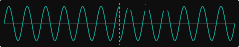
The simplified MS Hamiltonian is:
\[H_{\mathrm{PM}}(t)=\hbar g S_x \left(ae^{i[\delta t+\phi(t)]}+a^\dagger e^{-i[\delta t+\phi(t)]}\right)\]-
g is the spin-motion coupling strength
-
\(S_x\) is the collective spin operator
-
\(\delta\) is the detuning from the motional sideband
-
\(\phi\) is the phase of the laser
For PM gates \(\phi\) is modulated. This changes the direction of motion in phase space.
Use PM gates when you have precise phase control and want phase space trajectory engineering. Useful for composite pulse sequences, multimode decoupling and robust gates. Phase jumps can be implemented digitally and quickly. Scaling is a huge limiation to this. This is a lot easier than AM gates. Phase is far easier to change than amplitude.
Note:
Some configurations do several short pulses with alternating phases instead of straight phase modulation.
- \(R_0\)
-
Then \(R_{d1}\) so mode 1 closes. And so on.
-
Every application of \(R_d\) dpib;es the sequence (\(2^{M}-1\) phase shifts and \(2^M\) intevals)
-
As you concatenate intervals it supresses higher order noise sources. Things like detuning error, laser fluctuations, and variations in coupling strength are supressed.
-
Used for multimode oscillator closure AND high-order noise supression
AM Gates
Amplitude Modulated Gates.
If we modulate the amplitude of the gate beam we can cancel out spectator modes close to resonance.
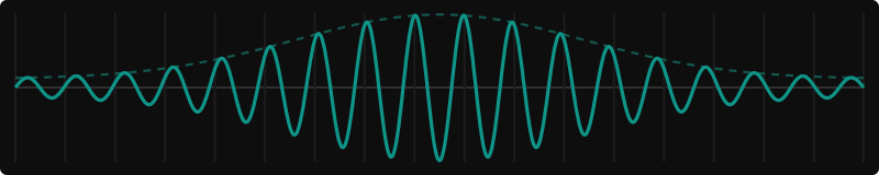
The simplified MS Hamiltonian is:
\[H_{\mathrm{PM}}(t)=\hbar g S_x \left(ae^{i[\delta t+\phi(t)]}+a^\dagger e^{-i[\delta t+\phi(t)]}\right)\]-
g is the spin-motion coupling strength
-
\(S_x\) is the collective spin operator
-
\(\delta\) is the detuning from the motional sideband
-
\(\phi\) is the phase of the laser
For AM gates g is modulated. This changes how quickly the ion moves in phase space.
If we modulate the amplitude of the gate beam we can cancel out spectator modes close to resonance. By shaping laser amplitude over time, you can arange for the unwanted motional displacements to cancel at the end of the gate.
It can also be used for pulse shaping - avoids sharper pulse edges.
Note:
If you modulate the amplitude at the trap frequency, it can be used as an AOM. The unmodulated laser field is:
\[E(t)=E_0\cos(\omega_L t)\]Amplitude modulating the laser field:
\[E(t)=E_0[1+m\cos(\omega_m t)]\cos(\omega_L t)\]Use the trig identity:
\[\cos A\cos B=\frac{1}{2}[\cos(A+B)+\cos(A-B)]\]Result:
\[\begin{aligned} E(t)={}&E_0\cos(\omega_L t)\\ &+\frac{mE_0}{2}\cos[(\omega_L+\omega_m)t]\\ &+\frac{mE_0}{2}\cos[(\omega_L-\omega_m)t] \end{aligned}\]
FM Gates
Frequency Modulated Gates.
If we modulate the frequency of the laser beam we can supress epectator modes and cause them to cancel to 0 at the end of the gate.
Noise that accumulates is reversed and cancels out as the frequency modulates.
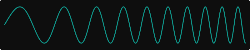
The simplified MS Hamiltonian is:
\[H_{\mathrm{PM}}(t)=\hbar g S_x \left(ae^{i[\delta t+\phi(t)]}+a^\dagger e^{-i[\delta t+\phi(t)]}\right)\]-
g is the spin-motion coupling strength
-
\(S_x\) is the collective spin operator
-
\(\delta\) is the detuning from the motional sideband
-
\(\phi\) is the phase of the laser
For FM gates \(\delta\) is modulated. This changes the direction the instantaneous trajectory bends in phase space.
FM gates are attractive for long chains. Many modes contribute to the interaction here. Modulating the frequency does so for all modes, and can thus close many modes at once.
Note:
FM and PM gates are closely related. Thedetuning is: \(\delta(t)=\delta_0+\Delta\cos(\omega_{\mathrm{mod}}t)\). And thus frequency modulation can be described as a time dependent phase.
The sidtinction is that FM gates specify the instantaneous frequency and change the instantaneous trajectory while PM gates often use discrete phase jumps.
Atomic Physics
Introduction
Basic Atomic Physics Intro.
Better Atomic Physics Intro
Standard references throughout: Foot, Atomic Physics; Metcalf & van der Straten, Laser Cooling and Trapping; Allen & Eberly, Optical Resonance and Two-Level Atoms.
Level structure
An atom’s electron can only be be certain distances away from its nucleus. like standing on the rungs of a ladder but never between them. Therefore, it can only have certain amounts of energy. These notes cover what decides where those rungs sit.
The big energy rungs come from the electron being pulled toward the nucleus. Smaller effects then split each rung into several closely spaced ones, and those small splittings turn out to matter a lot.
Each splitting below is a perturbation smaller than the one before it, so the good quantum numbers change down the hierarchy: \(n, l \to j \to F \to m_F\). When a perturbation stops being small compared with the one above it (strong external fields), the coupling order and the good quantum numbers change.
Overview: what splits the levels
If you look closely at an atom’s energy levels, most of them are not single lines but small bunches of lines. Several things cause this, from inside the atom, plus two that come from outside:
- Fine structure. The electron acts like a tiny magnet (it has “spin”), and as it moves around the nucleus it feels a magnetic field. Small effects from Einstein’s relativity add in too.
- Hyperfine structure. The nucleus is also a tiny magnet, even weaker. Its interaction with the electron makes an even finer split.
- Zeeman effect. Put the atom near an outside magnet and the levels split further, depending on how the atom’s tiny magnets point.
- Stark effect. Put the atom in an outside electric field and the levels shift, because the field stretches the atom.
The best quantum bit lives in one of these small splittings: the hyperfine one.
- Spin-orbit coupling. The electron’s spin couples to its orbital angular momentum.
- Fine structure. Three small corrections to the hydrogen levels: the relativistic kinetic energy, spin-orbit coupling and the Darwin term.
- Hyperfine structure. The electron’s magnetic field couples to the nucleus’s magnetic moment.
- Zeeman effect. The atom sits in an external magnetic field.
- Stark effect. The atom sits in an external electric field.
Scales. For hydrogen the gross structure is set by the Rydberg energy, \(E_n = -\tfrac12\alpha^2 m_ec^2/n^2\). Fine structure is smaller by \(\sim\alpha^2 \approx 5\times10^{-5}\). Hyperfine structure is smaller again by roughly \((m_e/m_p)\,g_I\), giving GHz-scale splittings (8.037 GHz for the Barium 137+ ground state). External fields add the Zeeman shift, \(\mu_B B/h \approx 1.40\) MHz/G for \(g = 1\), and the Stark shift, which is quadratic in \(E\) for any state without a degenerate partner of opposite parity.
For Ba\(^+\). Ba\(^+\) is alkali-like: one \(6s\) valance electron. The core screens and is penetrated by the valence electron, which lifts the \(l\)-degeneracy of hydrogen (quantum defects) and drops the \(5D\) levels below \(6P\). The scales are then: optical transitions \(\sim 600\) THz, \(6P\) fine structure \(\sim 51\) THz, \(5D\) fine structure \(\sim 25\) THz, ground-state hyperfine (for \(^{137}\)Ba\(^+\)) 8.037 GHz, and Zeeman splittings of MHz in a few-gauss field.
Fine structure
The simplest picture of hydrogen gives energy levels that depend only on which “shell” the electron is in. But, each level is split by a tiny amount, around a hundred-thousandth of the level’s energy or less. That is fine structure.
Three effects cause it:
- Relativity. Near the nucleus the electron moves fast enough that Einstein’s corrections to its energy matter a little.
- Spin-orbit coupling. From the electron’s point of view, the charged nucleus is circling around it. A moving charge makes a magnetic field, and the electron’s own spin acts as a tiny magnet too, and has slightly different energy depending on whether it lines up with that field or against it.
- The Darwin term. A subtle quantum effect that only matters for electrons whose cloud reaches right into the nucleus.
The result: levels that looked identical now have slightly different energies.
Small splittings of the hydrogen levels, of order \(\alpha^2\) relative to the Bohr energies \(E_n = -13.6\,\text{eV}/n^2\). They are the leading terms of a \(1/c^2\) expansion of the Dirac equation, and are treated in first-order perturbation theory in the \(|n,l,m_l\rangle\) basis (degenerate in \(l\), so in practice in the coupled \(|n,l,j,m_j\rangle\) basis, where all three terms are diagonal). They come from three terms:
- Relativistic kinetic energy. Expanding \(\sqrt{p^2c^2 + m^2c^4}\) beyond \(p^2/2m\) gives \[H_{\text{rel}} = -\frac{p^4}{8m^3c^2}.\] High-momentum states, which spend more time close to the nucleus, are pushed down in energy.
- Spin-orbit coupling. In the electron’s rest frame the nucleus orbits it, and that moving charge makes a magnetic field the electron’s spin feels: \[H_{SO} = \frac{1}{2m^2c^2}\,\frac{1}{r}\frac{dV}{dr}\,\vec L\cdot\vec S,\] where \(V(r)\) is the electron’s potential energy in the Coulomb field. Now \(j = l \pm \tfrac12\) states have different energies. Because \(\vec L\cdot\vec S = \tfrac12\left[J(J+1) - L(L+1) - S(S+1)\right]\) (in units of \(\hbar^2\)), \(H_{SO}\) is diagonal in \(|l,j,m_j\rangle\), which is why \(j\) becomes the good quantum number. For hydrogen \(\tfrac1r\tfrac{dV}{dr} = \tfrac{e^2}{4\pi\epsilon_0 r^3}\).
- Darwin term. Comes from the electron’s “jittery” motion, an interference between the positive- and negative-energy solutions of the Dirac equation. It only affects \(s\) states (\(l = 0\)), since they have weight at \(r = 0\): \[H_D = \frac{\hbar^2}{8m^2c^2}\nabla^2V = \frac{\pi\hbar^2}{2m^2c^2}\,\frac{e^2}{4\pi\epsilon_0}\,\delta^3(\vec r)\quad\text{(hydrogen)}.\]
All of these together give: \[\Delta E_{n,j} = E_n\,\frac{\alpha^2}{n^2}\left(\frac{n}{j + \tfrac12} - \frac34\right).\]
The \(l\)-dependence cancels between the three terms, so the result depends only on \(n\) and \(j\). This is the \(O(\alpha^2)\) expansion of the exact Dirac energy for a hydrogen-like ion of charge \(Z\): \[E_{nj} = mc^2\left[1 + \left(\frac{Z\alpha}{n - \delta_j}\right)^2\right]^{-1/2},\qquad \delta_j = j + \tfrac12 - \sqrt{\left(j + \tfrac12\right)^2 - Z^2\alpha^2}.\] So \(2S_{1/2}\) and \(2P_{1/2}\) stay degenerate.
Alkali-like ions. For a valence electron in a screened central potential the same spin-orbit form holds with \(V(r)\) replaced by the effective potential, so the splitting is dominated by the region near the nucleus where the screening fails and scales steeply with nuclear charge. That is why heavy ions like Ba\(^+\) have fine-structure splittings of tens of THz. A large fine-structure splitting matters for Raman gates: spin-flip Raman scattering is suppressed only for detunings comparable to or beyond it. Reference: Foot ch. 2 and 4; Bethe & Salpeter, Quantum Mechanics of One- and Two-Electron Atoms.
Hyperfine structure
The nucleus at the center of an atom can act like a very weak bar magnet. The electron makes its own magnetic field, and the energy depends on how the nucleus’s little magnet points relative to it, a bit like two compass needles that prefer certain arrangements.
That gives an even smaller split than fine structure, naturally called hyperfine structure. Fun fact that I think is cool: In hydrogen it produces the famous 21 cm radio line that astronomers use to map gas across the galaxy.
For ¹³⁷Ba⁺, the nucleus has a spin of 3/2 and the lowest energy level splits into two closely spaced levels, about 8 GHz apart in frequency. Those two levels are our qubit: one is called “0” and the other “1”. Because both are versions of the ground state, neither one decays on its own, which makes them very good at holding information. Hyperfine quibits are most popular for ions because of the clock transition. Going from \[F=1, m_j=0\] to \[F=2, m_j=0\], it is insensitive to the magnetic field.
Splittings from the interaction between the electron’s magnetic field and the nucleus’s magnetic moment. The nuclear spin \(\vec I\) and the electron angular momentum \(\vec J\) add to a total \(\vec F = \vec I + \vec J\), with \(F = |I - J|, \dots, I + J\): \[H_{HF} = A\,\vec I\cdot\vec J = \frac{A}{2}\Big[F(F+1) - I(I+1) - J(J+1)\Big],\] where \(A\) is the hyperfine coupling constant (here \(\vec I, \vec J\) are dimensionless, so \(A\) is an energy, usually quoted as \(A/h\) in MHz).
For hydrogen (\(I = J = \tfrac12\)), \(F = 1\) (a triplet) or \(F = 0\) (a singlet), and \[\Delta E_{HF} = \frac{A}{2}\left[F(F+1) - \frac32\right].\] The splitting is \(A\), the 1420.4 MHz (21 cm) line.
Where \(A\) comes from. For \(s\) electrons the dominant term is the Fermi contact interaction, \(A \propto g_I\,|\psi(0)|^2\), since only \(s\) states have density at the nucleus. For \(l > 0\) the orbital and spin-dipolar fields contribute instead, and \(A\) is much smaller. This is why \(S_{1/2}\) hyperfine splittings are GHz while \(P\) and \(D\) splittings are typically hundreds of MHz or less.
Interval rule. Adjacent levels are spaced by \(E(F) - E(F-1) = AF\). For \(J = \tfrac12\) there are only two levels, \(F = I \pm \tfrac12\), split by \[\Delta E_{HF} = A\left(I + \tfrac12\right).\]
Electric quadrupole term. For \(I \ge 1\) and \(J \ge 1\) the nucleus’s electric quadrupole moment couples to the electric-field gradient of the electron cloud, adding: \[H_Q = B\,\frac{3(\vec I\cdot\vec J)^2 + \tfrac32(\vec I\cdot\vec J) - I(I+1)J(J+1)}{2I(2I-1)\,J(2J-1)}.\] It vanishes for \(J = \tfrac12\), so the \(^{137}\)Ba\(^+\) \(S_{1/2}\) and \(P_{1/2}\) levels are pure magnetic-dipole, while \(P_{3/2}\), \(D_{3/2}\) and \(D_{5/2}\) need both \(A\) and \(B\) (and the interval rule is broken).
For \(^{137}\)Ba\(^+\) (\(I = 3/2\), \(J = 1/2\)) the ground state splits into \(F = 1\) and \(F = 2\), 8.037 GHz apart, so \(A_{S_{1/2}} = \Delta E_{HF}/2 \approx h\times 4018.87\) MHz. That splitting is the qubit. The \(F = 2\) level lies higher (positive \(A\)). Reference: Arimondo, Inguscio & Violino, Rev. Mod. Phys. 49, 31 (1977); Steck’s alkali notes for the formalism.
Zeeman effect
The atom contains tiny magnets: the electron’s orbit, the electron’s spin and the nucleus. Put the atom in an outside magnetic field and each energy level splits into several, depending on how those magnets are tilted relative to the field. It is like a compass needle: pointing with the field is low energy, pointing against it is high energy, and quantum mechanics only allows a few tilts in between. The direction you tilt the field in the lab definitely matters here.
How it looks depends on how strong the field is:
- Weak field. Each level splits into a neat set of evenly spaced sublevels. This is the usual case in the lab.
- Medium field. The levels start to mix and the spacing stops being even.
- Strong field. The outside field is so big it dominates. It just wins over the atom’s internal magnetism, and the electron’s spin and orbit respond to it separately.
We almost always apply a small magnetic field. It gives the atom a definite “up” direction and lets us pick out individual sublevels.
Splitting of levels in an external magnetic field \(\vec B_0 = B_0\hat z\): \[H_Z = -\vec B_0\cdot(\vec\mu_L + \vec\mu_S + \vec\mu_I) \approx \omega_L(L_z + 2S_z) + \omega_n I_z,\] with \(\omega_L\) and \(\omega_n\) the Larmor frequencies of the electron and the nucleus (\(\omega_L \gg |\omega_n|\); the “2” is \(g_s \approx 2.0023\)). The full Hamiltonian is the fine/hyperfine part plus \(H_Z\), and optical transitions obey \(\Delta m = 0, \pm 1\).
- Weak field (spin-orbit \(\gg\) Zeeman): \(J\) stays a good quantum number and each level splits into \(2J+1\) equally spaced sublevels.
- Intermediate field (spin-orbit \(\sim\) Zeeman): the states mix, \(J\) is no longer a good quantum number, and the level shifts are nonlinear in \(B\).
- Strong field Zeeman \(\gg\) spin-orbit): \(L\) and \(S\) decouple, the good quantum numbers are \(m_L, m_S\), and \[\Delta E = \mu_B B\,(m_L + g_s m_S).\]
Landé factors (weak field). By the projection theorem, within a \(J\) manifold \(\langle L_z + g_sS_z\rangle = g_J m_J\), so \(\Delta E = g_J\mu_B B\,m_J\) with \[g_J \approx 1 + \frac{J(J+1) + S(S+1) - L(L+1)}{2J(J+1)}\qquad (g_s \to 2).\] So \(g_J = 2\) for \(S_{1/2}\), \(2/3\) for \(P_{1/2}\), \(4/3\) for \(P_{3/2}\), \(4/5\) for \(D_{3/2}\) and \(6/5\) for \(D_{5/2}\). The same argument one level down, when the Zeeman energy is small compared with the hyperfine splitting, gives \(\Delta E = g_F\mu_B B\,m_F\) with \[g_F \approx g_J\,\frac{F(F+1) + J(J+1) - I(I+1)}{2F(F+1)}\] For the \(^{137}\)Ba\(^+\) ground state, \(g_F = +\tfrac12\) for \(F = 2\) and \(-\tfrac12\) for \(F = 1\): the \(m_F = \pm1\) states move by about \(\pm 0.70\) MHz/G.
Hyperfine intermediate field For \(J = \tfrac12\) the hyperfine-plus-Zeeman Hamiltonian is exactly solvable at any field. With \(\Delta E_{HF} = A(I + \tfrac12)\) and \(H_Z = \mu_B(g_JJ_z + g_II_z)B\), \[E_{F = I\pm\frac12,\,m} = -\frac{\Delta E_{HF}}{2(2I+1)} + g_I\mu_B m B \pm \frac{\Delta E_{HF}}{2}\sqrt{1 + \frac{4mx}{2I+1} + x^2},\qquad x = \frac{(g_J - g_I)\mu_B B}{\Delta E_{HF}}.\]
Clock states and the quadratic Zeeman shift. For \(m = 0\) the linear term in \(x\) drops out, and the qubit frequency is \(\Delta E_{HF}\sqrt{1 + x^2}/h\). To lowest order \[\nu_{\text{clock}}(B) \approx \nu_{HF} + K B^2,\qquad K = \frac{\left[(g_J - g_I)\mu_B/h\right]^2}{2\nu_{HF}}.\] A 1 mG field fluctuation shifts the qubit by about 5 Hz. Compare about 1.4 MHz/G for a first-order-sensitive \(\Delta m_F = \pm 1\) transition. That factor of \(\sim 300\) is why the \(m_F = 0\) pair is used and called a “clock state”. Reference: Breit & Rabi, Phys. Rev. 38, 2082 (1931); Foot ch. 6.
Stark effect
An electric field pulls the positive nucleus one way and the negative electron the other way, stretching the atom slightly. That changes the energy levels. This is the Stark effect.
In ion traps, lasers make electric fields too, so a laser can shift an ion’s levels this way. That “light shift” is useful (it is how optical tweezers grab atoms) and is also something we have to correct for.
Shift of energy levels in an external electric field, \(H = e E z\).
- Ground state (\(n = 1\)). The first-order shift is zero (the state has no permanent dipole moment). The second-order shift is negative, so the level is pushed down.
- \(n = 2\). There are four degenerate states \(|n,l,m\rangle\): \(|200\rangle, |210\rangle, |211\rangle, |21{-1}\rangle\). The field only couples states with \(\Delta l = \pm1\) and \(\Delta m = 0\), so only \(|200\rangle\) and \(|210\rangle\) mix. They split linearly in the field: \[E = E_2 \pm 3eEa_0,\] with \(a_0\) the Bohr radius. \(|211\rangle\) and \(|21{-1}\rangle\) are unshifted at first order.
Why first order vanishes. \(z\) is odd under parity, and every non-degenerate state has definite parity, so \(\langle\psi|z|\psi\rangle = 0\). A linear Stark effect needs degenerate states of opposite parity, which is special to hydrogen. Atoms and ions like Ba\(^+\) have only a quadratic Stark effect.
Quadratic Stark shift and polarizability. Second-order perturbation theory gives \[\Delta E_g = \sum_{k\neq g}\frac{|\langle k|eEz|g\rangle|^2}{E_g - E_k} \equiv -\frac12\,\alpha_0\,E^2,\] which defines the static polarizability \(\alpha_0 > 0\) for the ground state (every term is negative). For hydrogen \(\alpha_0 = \tfrac92\,(4\pi\epsilon_0)a_0^3\). For \(J \ge 1\) the polarizability has a tensor part that depends on \(m_J\) relative to \(\vec E\); for \(J = \tfrac12\) it vanishes.
AC Stark shift (light shift). For an oscillating field \(E(t) = E_0\cos(\omega t)\) far from resonance, the time-averaged shift is \[\Delta E = -\frac14\,\alpha(\omega)E_0^2 = -\frac{\alpha(\omega)\,I}{2\epsilon_0c},\qquad \alpha(\omega) = \frac{2}{\hbar}\sum_k\frac{\omega_{kg}\,|\langle k|d_z|g\rangle|^2}{\omega_{kg}^2 - \omega^2},\] with \(\omega_{kg} = (E_k - E_g)/\hbar\) and \(I = \tfrac12c\epsilon_0E_0^2\). Below all resonances \(\alpha > 0\) and the light attracts the atom to high intensity (red-detuned optical tweezers). Between resonances \(\alpha(\omega)\) changes sign, and zeros of \(\alpha\) are tune-out wavelengths. For a two-level atom in the RWA this reduces to \(\Delta E_g = \hbar\Omega^2/4\Delta\) with \(\Delta = \omega - \omega_0\). For circular or elliptical polarization there is also a vector light shift, proportional to \(i(\hat\epsilon^*\times\hat\epsilon)\), which acts like a fictitious magnetic field along the beam; the Raman polarization rule in the Ion Trapping notes is a consequence of it.
Why it matters in a trap. A trapped ion sits where the time-averaged force vanishes, not necessarily where the RF field vanishes. Excess micromotion means the ion samples the RF field, which gives a quadratic Stark shift \(\propto\langle E_{rf}^2\rangle\) (one of the leading systematics in ion clocks). Blackbody radiation shifts levels the same way, with \(\langle E^2\rangle \approx (8.32\ \text{V/cm})^2(T/300\,\text{K})^4\). For a hyperfine clock qubit both hyperfine levels have almost the same polarizability, so static Stark shifts of the qubit frequency are tiny; light shifts from gate beams are not, and must be calibrated or cancelled. Reference: Foot ch. 2 and 9; Grimm, Weidemüller & Ovchinnikov, Adv. At. Mol. Opt. Phys. 42, 95 (2000) for optical dipole potentials.
A two-level atom and light
Real atoms have many levels, but often a laser only connects two of them. Treating the atom as a simple two-level system, like a coin that can be heads or tails or something in between, explains most of what we do.
Truncating to two levels is valid when one transition is near-resonant and every other is far detuned compared with the Rabi frequency. The field is treated classically. Coherent dynamics follow from the Schrödinger equation in the rotating-wave approximation, and spontaneous emission and dephasing enter through the optical master equations.
Two-level Hamiltonian
The “Hamiltonian” is just physicist language for energy of a state, which then tells you how the system changes in time.
For a two-level atom it is very simple: there is a lower state (ground) and an upper state (excited), and the only thing that matters is the energy gap between them. That gap sets a frequency through
\[E = hf,\]where \(h\) is Planck’s constant, a tiny fixed number. A bigger energy gap means a higher frequency. To jump from the lower state to the upper one, the atom has to absorb light whose frequency matches that gap, like a radio that only picks up one station.
For our barium qubit the gap corresponds to about 8 GHz, a microwave frequency a bit above Wi-Fi.
With ground state \(|g\rangle\) and excited state \(|e\rangle\), \[H^{(e)} = \hbar\left(\omega_g|g\rangle\langle g| + \omega_e|e\rangle\langle e|\right) = \hbar\frac{\omega_e + \omega_g}{2}\,\mathbb 1 + \hbar\frac{\omega}{2}\Big(|e\rangle\langle e| - |g\rangle\langle g|\Big),\] with \(\omega = \omega_e - \omega_g\). Dropping the constant offset, \[H^{(e)} = \frac{\hbar\omega}{2}\,\sigma_z,\qquad \sigma_z = |e\rangle\langle e| - |g\rangle\langle g|.\]
Operator algebra. Define \(\sigma_+ = |e\rangle\langle g|\), \(\sigma_- = |g\rangle\langle e|\), \(\sigma_x = \sigma_+ + \sigma_-\), \(\sigma_y = -i(\sigma_+ - \sigma_-)\). Any two-level system is formally a spin-\(\tfrac12\), and any Hamiltonian on it can be written \(H = \tfrac{\hbar}{2}(\Omega_0\mathbb 1 + \vec\Omega\cdot\vec\sigma)\).
Two-level atom in a laser field
When a laser hits an atom, three things are going on at once:
- the ion jiggling back and forth in the trap,
- the ion’s internal state (ground or excited),
- the laser, which links the two.
If the laser is tuned to the atom’s frequency, it pushes the atom smoothly from ground to excited and back again, over and over. This back-and-forth is called a Rabi oscillation, and how fast it happens is the Rabi frequency. Stronger laser, faster flipping. Think of pushing a swing at exactly its natural rhythm: each push adds up.
Light also carries a small push (momentum). So when the ion absorbs light, it gets a tiny kick, and that kick connects the ion’s internal state to its motion in the trap. That connection is the key to everything in the Ion Trapping section.
For a trapped ion the full Hamiltonian has three parts: \[H = H^{(m)} + H^{(e)} + H^{(i)},\] the motion in the trap, the internal states, and the interaction with the laser. The interaction is \[H^{(i)} = \frac{\hbar\Omega}{2}\left(\sigma_+ + \sigma_-\right)\left(e^{i(k\hat x - \omega t + \phi)} + \text{h.c.}\right),\] with \(\Omega\) the Rabi frequency, \(\sigma_+ = |e\rangle\langle g|\) and \(\sigma_- = |g\rangle\langle e|\).
The \(e^{ik\hat x}\) factor is what couples the internal state to the motion. See the Lamb-Dicke notes in the Ion Trapping section.
Approximations hidden in this form. (i) A classical, monochromatic field. (ii) The electric-dipole approximation: the field is taken constant over the electron’s orbit (\(ka_0 \ll 1\)), so the coupling is \(-\hat{\vec d}\cdot\vec E\). The plane-wave phase is kept at the ion’s centre-of-mass position \(\hat x\). (iii) Two levels: all other transitions are detuned by much more than \(\Omega\).
Rotating frame and RWA. Ignoring motion (\(k\hat x \to 0\)), go to the frame rotating at the laser frequency, \(U = e^{i\omega t\sigma_z/2}\). The terms \(\sigma_+e^{-i\omega t}\) become static and \(\sigma_+e^{+i\omega t}\) oscillate at \(2\omega\). Dropping the latter (rotating-wave approximation, valid for \(\Omega, |\Delta| \ll \omega\)) gives the time-independent \[H_{\text{RWA}} = -\frac{\hbar\Delta}{2}\sigma_z + \frac{\hbar\Omega}{2}\left(e^{i\phi}\sigma_+ + e^{-i\phi}\sigma_-\right),\qquad \Delta = \omega - \omega_0.\] This is a spin in an effective field \(\vec\Omega = (\Omega\cos\phi, \Omega\sin\phi, -\Delta)\): the laser phase sets the rotation axis in the equatorial plane and the detuning tilts it out of the plane.
Rabi formula. Starting in \(|g\rangle\), \[P_e(t) = \frac{\Omega^2}{\Omega^2 + \Delta^2}\,\sin^2\left(\frac{\Omega' t}{2}\right),\qquad \Omega' = \sqrt{\Omega^2 + \Delta^2}.\] On resonance, a pulse of area \(\theta = \Omega t\) rotates the Bloch vector by \(\theta\) (\(\pi\) pulse: full inversion; \(\pi/2\) pulse: equal superposition). Off resonance the oscillation is faster and incomplete.
Dressed states and light shifts. The eigenvalues of \(H_{\text{RWA}}\) are \(\pm\tfrac{\hbar}{2}\Omega'\). For \(|\Delta| \gg \Omega\) the state adiabatically connected to \(|g\rangle\) is shifted by \[\delta E_g = \frac{\hbar\Omega^2}{4\Delta},\] and \(|e\rangle\) by the opposite amount: the AC Stark shift. Red detuning (\(\Delta < 0\)) lowers the ground state. In a near-resonant strong field the fluorescence and absorption spectra split by \(\Omega'\). Reference: Allen & Eberly; Foot ch. 7; Steck, Quantum and Atom Optics.
Recoil. Each absorbed photon transfers momentum \(\hbar k\), i.e. a recoil energy \(\hbar\omega_R = \hbar^2k^2/2m\). In a trap of frequency \(\nu\) the ratio \(\omega_R/\nu = \eta^2\) is the square of the Lamb-Dicke parameter, which is where the \(e^{ik\hat x}\) factor enters the physics.
Scattering rate
Placeholder
Placeholder
T1 time
T1 is how long, on average, a qubit stays in its “1” state before it falls back to “0” on its own. It measures energy loss: the atom gives its extra energy to the surroundings, like a spinning top that slowly runs down.
The average time before the excited state decays due to coupling to the environment. It leaves the qubit space and decays to the ground state.
This is the length of the Rabi Oscillation.
T2 time
A qubit can be in a mix of “0” and “1” at the same time, called a superposition. That mix has a timing, or phase, between its two parts, like two clocks that tick together. T2 is how long that timing stays well defined.
How long a superposition maintains its phase coherence between \(|0\rangle\) and \(|1\rangle\). It stays in the qubit stapce, but loses its coherence.
This is the slope of the Rabi Oscillation.
Ramsey experiment
This is how you measure T2 time.
A Ramsey experiment is when you put the qubit into a superposition, then wait a bit, and then take it out of the superposition. Ideally it would be the same at the end, but it usually isn’t. It usually picks up a phase during the wait. By doing this multiple times and varying how long you wait you can see fringes. These fringes is the phase stability.
1: A \(\frac{\pi}{2}\) puts the qubit into superposition.
2: Free evolution of time gives realtitive phase \[\frac{1}{\sqrt{2}}(|g\rangle + e^{i\phi}|e\rangle)\] with \(\phi = \delta T\) with \(\delta\) = detuning.
3: A second \(\frac{\pi}{2}\) converts the accumulated phase into measurable population difference.
By varying T, the probability of a qubit being in the excited state oscillates \[P_e = \frac{1}{\sqrt{2}}[1+cos(\delta T]\]. The interference pattern (Ramsey Fringes) are sharpest when:
- Coherent evolution is maintained
- Phase stability is high
- Decoherence is minimal
Quantum Computing
Introduction
Placeholder
Placeholder
Quantum Computing Overview
What changed in 20th-century physics, and why quantum hardware is hard
Placeholder
Placeholder
Classical vs quantum information: bits, qubits and quantum advantage
Placeholder
Placeholder
The Rules
States, superposition, measurement and the Born rule
Placeholder
Placeholder
Unitary evolution, reversibility and no-cloning
Placeholder
Placeholder
One qubit
Bloch sphere and Pauli matrices
Placeholder
Placeholder
Single-qubit gates (X, Y, Z, H, S, T, rotations) and how a Raman pulse implements them
Placeholder
Placeholder
Many qubits
Tensor products and why the state space grows as 2ⁿ
Placeholder
Placeholder
Entanglement, Bell states and GHZ states
Placeholder
Placeholder
Two-qubit gates: CNOT, CZ, XX (MS), and converting between them
Placeholder
Placeholder
Universality and circuits
Universal gate sets and Solovay–Kitaev
Placeholder
Placeholder
Circuit notation, native trapped-ion gates (R(θ,φ) + MS) and compiling to them
Placeholder
Placeholder
Core protocols
Teleportation, superdense coding and entanglement swapping
Placeholder
Placeholder
Phase kickback
Placeholder
Placeholder
Algorithms
Deutsch and Deutsch–Jozsa
Placeholder
Placeholder
Simon's period finding
Placeholder
Placeholder
Quantum Fourier transform and Shor's factoring
Placeholder
Placeholder
Grover's search
Placeholder
Placeholder
Variational algorithms (VQE and QAOA) for near-term machines
Placeholder
Placeholder
Quantum state purification
Placeholder
Placeholder
Classical Optics
Introduction
Placeholder
Placeholder
RF Electronics
Introduction
Placeholder
Placeholder
Super Basics
Introduction
Placeholder
Placeholder
Optical Qubit
Uses two different energy levels as the \(|0\rangle\) and \(|1\rangle\) states.
For example:
In Ba 138+, the \(S\frac{1}{2}\) is typically chosen as \(|0\rangle\) and \(D\frac{3}{2}\) is typically \(|1\rangle\).
Uses two different energy levels as the \(|0\rangle\) and \(|1\rangle\) states. Thse have a large energy splitting, far more than hyperfine qubits.
Advangtages:
-
Direct transition - a laser can shift between states with precise control
-
Long lived metastable state
-
Avoids need for Raman or microwave gate
Disadvantages:
-
Finite lifetime on metastable state (most are incredibly long however)
-
Laser must have good frequency stability with respect to transition (Ba 138+ 1762nm transition linewidth is mHz)
-
Optical path length fluctuations can introduce phase noise
Hyperfine Qubit
In spin ions with a nuclear spin the ground state is split. Hyperfine qubits use two of those ground state levels as the \(|0\rangle\) and \(|1\rangle\) states.
For Ba 137+, the \(|S\frac{1}{2}, F=1, m+F=0 \rangle\) state is typically the \(|0\rangle\) state, and \(|S\frac{1}{2}, F=2, m+F=0 \rangle\) state is typically the \(|1\rangle\) state.
These are both in the ground state, so they do not decay and are magnetic field insensitive to the first order.
In spin ions with a nuclear spin the ground state is split. Hyperfine qubits use two of those ground state levels as the \(|0\rangle\) and \(|1\rangle\) states.
Advantages:
-
Both qubits tate can lie in the ground state manifold, so it avoids spontaneous decay
-
Hyperfine transitions are magnetic field insensitive to the first order
-
Microwave based gates give excellent frequency stability
-
Hyperfine qubits have very long coherence times
Disadvantages:
-
Splitting is far too small for lasers (GHz) - must use microwaves or Raman
-
Microwaves can not be focused down to hit an individual ion without hitting its neighbor (this is wavelenth dependent)
-
Microwave radiation coples weakly to the ion, so gates require additional techniques like magnetic field gradients
-
Raman gates can introduce sponatneous photon scattering
-
Raman transitions require precise laser control
OMG Qubit
Optical, Metastable, Ground state qubits.
OMG qubits are 3 qubits in one. It is an attempt to use both techniques of hyperfine qubits and optical qubits.
-
Sublevels of the groundstate act as a qubit
-
Whether it is in the ground state or metastable state act as another qubit
-
Sublevels in the metastable state act as a third qubit.
Optical, Metastable, Ground state qubits.
OMG qubits are 3 qubits in one. It is an attempt to use both techniques of hyperfine qubits and optical qubits.
-
Sublevels of the groundstate act as a qubit
-
Whether it is in the ground state or metastable state act as another qubit
-
Sublevels in the metastable state act as a third qubit.
The biggest motivation for OMG qubits is that conventional trapped ion quantum computers often use two different ion species. One to store info and one for sympathetic cooling. OMG tries to accomplish both with one ion species.
The ground state can scatter photons during laser cooling, while the metastable ions remain largely unaffected because their relavent transitions are far from the cooling transition. This makes it possible to cool the motion without “necessarily” destroying the stored info in other states.
Parts of this have been shown experimentally, but not all of it in one.
Barium: isotopes and nuclear spins
Barium atoms all have 56 protons, but different versions, called isotopes, have different numbers of neutrons. The number after “Ba” counts protons plus neutrons.
The nucleus can act like a tiny spinning magnet, and its “nuclear spin” sets whether the electron’s ground level gets split by hyperfine structure:
- Barium-138: nuclear spin 0. The most common kind, about 72% of natural barium. No nuclear magnetism, so no hyperfine split. Easy to work with but not useful as this kind of qubit.
- Barium-137: nuclear spin 3/2. About 11% of natural barium. Its ground level splits into two levels 8.037 GHz apart, and those form our qubit.
- Barium-133: nuclear spin 1/2. Also has a hyperfine qubit, with a simpler structure, but it is radioactive and has to be made artificially.
| Isotope | Nuclear spin \(I\) | Notes |
|---|---|---|
| \(^{138}\)Ba\(^+\) | \(0\) | Most abundant. No hyperfine structure. |
| \(^{137}\)Ba\(^+\) | \(3/2\) | Ground-state hyperfine \(F = 1, 2\) (8.037 GHz). Our qubit. |
| \(^{133}\)Ba\(^+\) | \(1/2\) | Radioactive. Ground-state hyperfine \(F = 0, 1\). |
Abundances. Natural barium is about 71.7% \(^{138}\)Ba and 11.2% \(^{137}\)Ba, with \(^{136}\)Ba, \(^{135}\)Ba and \(^{134}\)Ba making up most of the rest. \(^{135}\)Ba is the other stable odd isotope, also with \(I = 3/2\). \(^{133}\)Ba has a half-life of about 10.5 years.
Why the nuclear spin matters. Even isotopes (\(I = 0\)) have no hyperfine structure: simple to cool and detect, but the only qubits are Zeeman qubits (first-order field-sensitive) or optical (\(S\)–\(D_{5/2}\)) qubits. Odd isotopes have \(F = I \pm \tfrac12\) ground levels with field-insensitive \(m_F = 0\) clock pairs.
- \(I = 1/2\) (\(^{133}\)Ba\(^+\)): same structure as \(^{171}\)Yb\(^+\). The \(F = 1 \to F' = 0\) transition on \(S_{1/2}\to P_{1/2}\) is a closed cycling transition (the \(F' = 0\) state can only decay to \(F = 1\)), which allows direct hyperfine-selective fluorescence detection, and state preparation into \(|F = 0, m_F = 0\rangle\) is a single optical-pumping step. The cost is handling a radioactive source.
- \(I = 3/2\) (\(^{137}\)Ba\(^+\)): the \(P_{1/2}\) level has \(F' = 1, 2\), so there is no closed transition from either ground level; every excitation from \(F = 2\) can decay to \(F = 1\). Direct fluorescence detection therefore pumps the qubit before enough photons are collected, and detection is done by shelving one qubit state to \(D_{5/2}\) (see the levels note). The larger \(F\) also means more Zeeman sublevels to optically pump through.
Isotope-selective loading. Neutral Ba is ionized in two steps, resonantly on the 553.5 nm \(6s^2\,{}^1S_0 \to 6s6p\,{}^1P_1\) line and then with a photon shorter than about 417 nm to the continuum (the ionization energy is 5.21 eV). The isotope shifts and hyperfine structure of the first step provide selectivity; because \(^{137}\)Ba is only 11% of the natural mix, enriched sources help.
Laser consequences for \(^{137}\)Ba\(^+\). Every level has hyperfine structure, so cooling needs sidebands: the 493 nm light must address both \(F = 1\) and \(F = 2\) ground levels (an EOM at the 8.037 GHz splitting, or near it), and the 650 nm repump must address the hyperfine levels of \(D_{3/2}\) (\(F = 0\) to \(3\)).
Barium ion: levels and transitions
Placeholder
Placeholder
Hyperfine structure and ¹³⁷Ba⁺ qubit details
Placeholder
Placeholder
Gates
Introduction
A normal computer bit can be either 0 or 1.
A qubit can be in a state \(|0\rangle\), state \(|1\rangle\), or a superpositiob of both:
\[|\psi\rangle = \alpha|0\rangle + \beta|1\ranlge\]We can visualize a qubit as an arrow pointing somwehre on a sphere called the Bloch Sphere:
INSERT BLOCH SPHERE PICTURE
Every “gate” we talk about can be visualized as just a rotation on this sphere
A normal computer bit can be either 0 or 1.
A qubit can be in a state \(|0\rangle\), state \(|1\rangle\), or a superpositiob of both:
\[|\psi\rangle = \alpha|0\rangle + \beta|1\ranlge\]We can visualize a qubit as an arrow pointing somwehre on a sphere called the Bloch Sphere:
INSERT BLOCH SPHERE PICTURE
Every “gate” we talk about can be visualized as just a rotation on this sphere
X Gate
Swaps the bit from a 0 to 1 or 1 to 0.
On the Bloch Sphere, the arrow rotates around the X axis by 180 degrees.
Swaps the bit from a 0 to 1 or 1 to 0.
X \(|0\rangle\) = \(|1\rangle\)
X \(|1\rangle\) = \(|0\rangle\)
The Pauli X matrix is:
\begin{pmatrix} 0 & 1 \ 0 & 0 \end{pmatrix}
On the Bloch Sphere, the arrow rotates around the X axis by 180 degrees.
Y Gate
The Y gate also flips \(|0\rangle\) and \(|1\rangle\), but it introduces a phase too.
On the Bloch Sphere, the arrow rotates around the Y axis by 180 degrees.
This gate will be the same if the qubit starts in \(|0\rangle\), but not if it starts in a superposition. For example:
\[|+\ranlge = \frac{|0\rangle _ |1\rangle}{2}\]X \(|+\rangle\) = \(|+\ranlge\)
Y \(|+\rangle\) = \(-i|-\rangle\)
The Y gate also flips \(|0\rangle\) and \(|1\rangle\), but it introduces a phase too.
Y \(|0\rangle\) = \(i|1\rangle\)
Y \(|1\rangle\) = \(-i|0\rangle\)
The Pauli Y matrix is:
\begin{pmatrix} 0 & i \ -i & 0 \end{pmatrix}
On the Bloch Sphere, the arrow rotates around the Y axis by 180 degrees.
Z Gate
The Z gate changes the pphase of a qubit without changing the probability its in a \(|0\rangle\) or \(|1\rangle\) state.
It is a rotation on the Bloch sphere around the Z axis by 180 degrees.
The Z gate changes the pphase of a qubit without changing the probability its in a \(|0\rangle\) or \(|1\rangle\) state.
The Pauli Z matrix is:
\begin{pmatrix} 1 & 0 \ 0 & -1 \end{pmatrix}
It is a rotation on the Bloch sphere around the Z axis by 180 degrees.
H Gate
This puts the qubit that is definitely in a \(|0\rangle\) or \(|1\rangle\) state and puts it into a superposition
H \(|0\rangle\) = \(|+\rangle\)
H \(|1\rangle\) = \(|-\rangle\)
It is a rotation on the Bloch sphere of 180 dgrees along an axis halfway between the X and Z axis.
This puts the qubit that is definitely in a \(|0\rangle\) or \(|1\rangle\) state and puts it into a superposition
The Pauli H matrix is:
\(\frac{1}{\sqrt{2}}\) \begin{pmatrix} 1 & 1 \ 1 & -1 \end{pmatrix}
It is a rotation on the Bloch sphere of 180 dgrees along an axis halfway between the X and Z axis.
s Gate
An S gate changes the relative phase of a qubit by a 90 degrees. It is a quarter turn phase gate.
S \(|0\rangle\) = \(|0\rangle\)
S \(|1\rangle\) = \(i|1\rangle\)
An S gate changes the relative phase of a qubit by a 90 degrees. It is a quarter turn phase gate.
The Pauli S matrix is:
\begin{pmatrix} 1 & 0 \ 0 & i \end{pmatrix}
It is a rotation on the Bloch sphere of 90 dgrees along the Z axis.
T Gate
A T gate changes the relative phase of a qubit by a 45 degrees. It is an eigth turn phase gate.
S \(|0\rangle\) = \(|0\rangle\)
S \(|1\rangle\) = \(e^{i\frac{\pi}{4}}|1\rangle\)
A T gate changes the relative phase of a qubit by a 45 degrees. It is an eigth turn phase gate.
The Pauli T matrix is:
\begin{pmatrix} 1 & 0 \ 0 & e^{i\frac{\pi}{4}} \end{pmatrix}
It is a rotation on the Bloch sphere of 45 dgrees along the Z axis.
CNOT Gate
This is a 2 qubit gate. If the control qubit is 1 then the target qubit flips. If the control qubit is 0 then nothing happens.
-
\(|00\rangle\) -> \(|00\rangle\)
-
\(|01\rangle\) -> \(|01\rangle\)
-
\(|10\rangle\) -> \(|11\rangle\)
-
\(|11\rangle\) -> \(|10\rangle\)
This is a 2 qubit gate. If the control qubit is 1 then the target qubit flips. If the control qubit is 0 then nothing happens.
The Pauli CNOT matrix is:
\begin{pmatrix} 1 & 0 & 0 & 0 \ 0 & 1 & 0 & 0 \ 0 & 0 & 0 & 1 \ 0 & 0 & 1 & 0 \end{pmatrix}
-
\(|00\rangle\) -> \(|00\rangle\)
-
\(|01\rangle\) -> \(|01\rangle\)
-
\(|10\rangle\) -> \(|11\rangle\)
-
\(|11\rangle\) -> \(|10\rangle\)
CZ Gate
This is a 2 qubit gate. If the control qubit is 1 then the phase of the target qubit flips. If the control qubit is 0 then nothing happens.
-
\(|00\rangle\) -> \(|00\rangle\)
-
\(|01\rangle\) -> \(|01\rangle\)
-
\(|10\rangle\) -> \(|10\rangle\)
-
\(|11\rangle\) -> \(-|11\rangle\)
This is a 2 qubit gate. If the control qubit is 1 then the phase of the target qubit flips. If the control qubit is 0 then nothing happens.
The Pauli CZ matrix is:
\begin{pmatrix} 1 & 0 & 0 & 0 \ 0 & 1 & 0 & 0 \ 0 & 0 & 1 & 0 \ 0 & 0 & 0 & -1 \end{pmatrix}
-
\(|00\rangle\) -> \(|00\rangle\)
-
\(|01\rangle\) -> \(|01\rangle\)
-
\(|10\rangle\) -> \(|10\rangle\)
-
\(|11\rangle\) -> \(-|11\rangle\)
SWAP Gate
This is a 2 qubit gate. It just swaps the state of the two qubits.
-
\(|00\rangle\) -> \(|00\rangle\)
-
\(|01\rangle\) -> \(|10\rangle\)
-
\(|10\rangle\) -> \(|01\rangle\)
-
\(|11\rangle\) -> \(|11\rangle\)
It is done by applying 3 CNOT gates. CNOT(1,2)CNOT(2,1)CNOT(1,2)
This is a 2 qubit gate. It just swaps the state of the two qubits.
The Pauli SWAP matrix is:
\begin{pmatrix} 1 & 0 & 0 & 0 \ 0 & 0 & 1 & 0 \ 0 & 1 & 0 & 0 \ 0 & 0 & 0 & 1 \end{pmatrix}
-
\(|00\rangle\) -> \(|00\rangle\)
-
\(|01\rangle\) -> \(|10\rangle\)
-
\(|10\rangle\) -> \(|01\rangle\)
-
\(|11\rangle\) -> \(|11\rangle\)
It is done by applying 3 CNOT gates. CNOT(1,2)CNOT(2,1)CNOT(1,2)
Toffoli Gate
Just a CCNOT gate. A CNOT with an extra control
-
\(|110\rangle\) -> \(|111\rangle\)
-
\(|111\rangle\) -> \(|110\rangle\)
Just a CCNOT gate. A CNOT with an extra control
-
\(|110\rangle\) -> \(|111\rangle\)
-
\(|111\rangle\) -> \(|110\rangle\)
Quantum Engineering with Atoms Notes
Chapter 1 - Classical Vectors vs. Quantum Operators
In classical physics there are observables like position and momentum. In quantum physics we construct analogous operators by defining the “vector operators”.
\[\hat{r} = \hat{x}_1 e_1 + \hat{x}_2 e_2 + \hat{x}_3 e_3\] \[\hat{p} = \hat{p}_1 e_1 + \hat{p}_2 e_2 + \hat{p}_3 e_3\]
Sometimes in quantum observables do not commute:
\[[\hat{x}_i,\hat{p}_i]=i\\hbar\delta_{ij}\]Different components of angular momentum do not commute. But even though \(\hat{L}_i\) does not commute with any other component of \(\hat{L}\), it does commute with \(\hat{L}^2\):
\[[\hat{L}_i,\hat{L}^2]=0\]Our commuting set of Hermitian operators is \(\hat{H}, \hat{L}_z, \hat{L}\).
In classical physics there are observables like position and momentum. In quantum physics we construct analogous operators by defining the “vector operators”.
\[\hat{r} = \hat{x}_1 e_1 + \hat{x}_2 e_2 + \hat{x}_3 e_3\] \[\hat{p} = \hat{p}_1 e_1 + \hat{p}_2 e_2 + \hat{p}_3 e_3\]
Sometimes in quantum observables do not commute:
\[[\hat{x}_i,\hat{p}_i]=i\\hbar\delta_{ij}\]The cross product obeys classical rules - the dot product does not.
Angular momentm \(\hat{L}\) is Hermition.
\[\hat{L}^{\dagger} = \hat{L}\]Therefore it’s eigenvectors are orthogonal.
Different components of angular momentum do not commute. But even though \(\hat{L}_i\) does not commute with any other component of \(\hat{L}\), it does commute with \(\hat{L}^2\):
\[[\hat{L}_i,\hat{L}^2]=0\]Leet’s now look at orbital angular momentum in context of central potenitals (only depends on r). The Hamiltonian in this case is:
\[\hat{H}=\frac{\hat{p}^2}{2m} + V(r)\] \[\hat{H}= \frac{-\hbar^2}{2m4} \frac{\partial^2}{\partial r^2} \frac{\hat{L}^2}{2m} + V(r)\]Our commuting set of Hermitian operators is \(\hat{H}, \hat{L}_z, \hat{L}\).
Let’s define:
\[\hat{J}_{\pm} = \hat{J}_x \pm i\hat{J}_y\]It follows that:
\[[\hat{J}_{\pm},\hat{J}^2]=0\]Chapter 2 - The Hydrogen Atom
Central potential problems are ones where the potential only relys on distance from center (like electron and nucleus Coulomb field).
We can deal with these best in spherical coordiantes:
The Hamiltonian for a Central potential V(r) is:
\[\hat{H} = \frac{\hat{p}_r^2}{2mr} + \frac{\hat{L}^2}{2mr^2} _ V(r)\]We can use separation of variables to get terms that only rely on r and \(\theta\) and \(\phi\).
\[\hat{H} = R_{kl}(r)Y_l^m(\theta,\phi)\]Let’s now try to solve the Time Independent Schrodinger Equation (the solution is just a linear combo of plane waves in cartesian coordinates, but this is spherical coordinates):
\[\hat{H}\psi_{klm}(r,\theta,\phi) = E_{klm}\psi_{klm}(r,\theta,\phi) = E_{klm}R_{kl}(r)Y_l^m(\theta,\phi)\]Which has the solution:
\[\psi_{klm}(r,\theta,\phi) = j_l(kr)Y_l^m(\theta,\phi)\]Where \(j_l(kr)\) is a bessel function of the first kind. Upon measurement of energy, \((\hat{L}^2\)\) and \((\hat{L}_z\)\), the wavefunction yields \((E_k\)\), \((l(l+1)\hbar^2\)\) and \((m\hbar\)\), respectively.
A hydrogen atom is a negatively charged electron around a positively charged nucleus.
\[\hat{H} = \frac{\hat{p}_1^2}{2m_1} + \frac{\hat{p}_2^2}{2m_2} + V(|\vec{r}_1-\vec{r}_2|)\]This can be simplifeid to The center of mass Hamiltonian and relativistic Hamiltonian:
\[\hat{H}_{CM} = \frac{\hat{P}^2}{2M}\] \[\hat{H}_{rel} = \frac{\hat{p}^2}{2\mu} + V(|r|)\] \[V(|r|) = \frac{-e^2}{r}\]We find the binding energy of the electron to the nucleus is quantized as:
\[E_n = -\frac{13.6 eV}{n^2}\]For a fixed n there are n possible values of the orbital angular momentum quantum number \(l = 0, 1, ..., n-1\).
For each l value there are \(2l+1\) distinct values of \(m = -l, ..., +l\). So the degeneracy of quantum states is \(n^2\).
The final wavefinction of the electron in a Hydrogen atom is:
\[\psi_{nlm}(r,\theta,\phi)= \sqrt{\left(\frac{2}{na_0}\right)^3\frac{(n-l-1)!}{2n[(n+l)!]^3}}\,e^{-\rho/2}\rho^lL_{n-l-1}^{2l+1}(\rho)Y_l^m(\theta,\phi),\]With \(\rho = 2\kappa_n r = \frac{2r}{a_0 n}\).
Central potential problems are ones where the potential only relys on distance from center (like electron and nucleus Coulomb field).
We can deal with these best in spherical coordiantes:
\[\begin{aligned} x &= r\sin\theta\cos\phi \\ y &= r\sin\theta\sin\phi \\ z &= r\cos\theta \end{aligned}\] \[\begin{aligned} r &= \sqrt{x^2+y^2+z^2} \\ \theta &= \arctan\left(\frac{\sqrt{x^2+y^2}}{z}\right) \\ \phi &= \arctan\left(\frac{y}{x}\right) \end{aligned}\]Thus, we can write the anglumar momentum operators as:
\[\begin{aligned} \hat{L}_x &= -i\hbar\left[y\frac{\partial}{\partial z} -z\frac{\partial}{\partial y}\right] \\ &= -i\hbar\left[ -\sin\phi\frac{\partial}{\partial\theta} -\cot\theta\cos\phi\frac{\partial}{\partial\phi} \right] \\[8pt] \hat{L}_y &= -i\hbar\left[z\frac{\partial}{\partial x} -x\frac{\partial}{\partial z}\right] \\ &= -i\hbar\left[ \cos\phi\frac{\partial}{\partial\theta} -\cot\theta\sin\phi\frac{\partial}{\partial\phi} \right] \\[8pt] \hat{L}_z &= -i\hbar\left[x\frac{\partial}{\partial y} -y\frac{\partial}{\partial x}\right] \\ &= -i\hbar\frac{\partial}{\partial\phi} \\[8pt] \hat{L}^2 &= \hat{L}_x^2+\hat{L}_y^2+\hat{L}_z^2 \\ &= -\hbar^2\left[ \frac{1}{\sin\theta} \frac{\partial}{\partial\theta} \left(\sin\theta\frac{\partial}{\partial\theta}\right) +\frac{1}{\sin^2\theta} \frac{\partial^2}{\partial\phi^2} \right] \end{aligned}\]The Hamiltonian for a Central potential V(r) is:
\[\hat{H} = \frac{\hat{p}_r^2}{2mr} + \frac{\hat{L}^2}{2mr^2} _ V(r)\]We can use separation of variables to get terms that only rely on r and \(\theta\) and \(\phi\).
\[\hat{H} = R_{kl}(r)Y_l^m(\theta,\phi)\]Whose solution is:
\[Y_l^m(\theta,\phi) = \sqrt{\frac{2l+1}{4\pi}\frac{(l-m)!}{(l+m)!}}\,P_l^m(\cos\theta)e^{im\phi}\]Let’s now try to solve the Time Independent Schrodinger Equation (the solution is just a linear combo of plane waves in cartesian coordinates, but this is spherical coordinates):
\[\hat{H}\psi_{klm}(r,\theta,\phi) = E_{klm}\psi_{klm}(r,\theta,\phi) = E_{klm}R_{kl}(r)Y_l^m(\theta,\phi)\]Which simplifies to:
\[\frac{d^2}{dx^2}R_l(x) + \frac{2}{x}\frac{d}{dx}R_l(x) + \left[1-\frac{l(l+1)}{x^2}\right]R_l(x)=0\]Which has the solution:
\[\psi_{klm}(r,\theta,\phi) = j_l(kr)Y_l^m(\theta,\phi)\]Where \(j_l(kr)\) is a bessel function of the first kind. Upon measurement of energy, \((\hat{L}^2\)\) and \((\hat{L}_z\)\), the wavefunction yields \((E_k\)\), \((l(l+1)\hbar^2\)\) and \((m\hbar\)\), respectively.
A hydrogen atom is a negatively charged electron around a positively charged nucleus.
\[\hat{H} = \frac{\hat{p}_1^2}{2m_1} + \frac{\hat{p}_2^2}{2m_2} + V(|\vec{r}_1-\vec{r}_2|)\]This can be simplifeid to The center of mass Hamiltonian and relativistic Hamiltonian:
\[\hat{H}_{CM} = \frac{\hat{P}^2}{2M}\] \[\hat{H}_{rel} = \frac{\hat{p}^2}{2\mu} + V(|r|)\] \[V(|r|) = \frac{-e^2}{r}\]The Schrodinger equation becomes:
\[\left[-\frac{\hbar^2}{2\mu}\left(\frac{1}{r}\frac{d}{dr}r\right)^2+\frac{\hbar^2 l(l+1)}{2\mu r^2}-\frac{e^2}{r}+E\right]R_{nl}(r)=0,\]The solution is:
\[u_{nl}(\rho) = e^{-\rho/2}\rho^{l+1}F(\rho)\]We polynomial expand \(F(\rho)\) and plug this into the original equation and simplify to get:
\[\rho\frac{d^2}{d\rho^2}F(\rho) + (2l+2-\rho)\frac{d}{d\rho}F(\rho) + (\lambda-l-1)F(\rho)=0\]This is the Laguerre equation. The solutiion is the associated Laguerre polynomial \(F(\rho) = L_{n-l-1}^{2l+1}(\rho)\) where \(\rho = 2\kappa_n r\) and \(\kappa_n = \frac{1}{a_0 n}\).
We define the principal quantum number \(n = i_{max} + l + 1 \geq 1\).
We find the binding energy of the electron to the nucleus is quantized as:
\[E_n = -\frac{13.6 eV}{n^2}\]For a fixed n there are n possible values of the orbital angular momentum quantum number \(l = 0, 1, ..., n-1\).
For each l value there are \(2l+1\) distinct values of \(m = -l, ..., +l\). So the degeneracy of quantum states is \(n^2\).
The final wavefinction of the electron in a Hydrogen atom is:
\[\psi_{nlm}(r,\theta,\phi)= R_{nl}(r)Y_l^m(\theta,\phi)= \frac{A_{nl}u_{nl}}{r}Y_l^m(\theta,\phi)= A_{nl}'e^{-\rho/2}\rho^l L_{n-l-1}^{2l+1}(\rho)Y_l^m(\theta,\phi)\]It is fully generalized as:
\[\psi_{nlm}(r,\theta,\phi)= \sqrt{\left(\frac{2}{na_0}\right)^3\frac{(n-l-1)!}{2n[(n+l)!]^3}}\,e^{-\rho/2}\rho^lL_{n-l-1}^{2l+1}(\rho)Y_l^m(\theta,\phi),\]With \(\rho = 2\kappa_n r = \frac{2r}{a_0 n}\).
Chapter 3 - Magnetic Moment
\(\hat{S}\) is the spin - an intrinsi internal degree of freedom that behaves exactly like angular momentum.
Similarly to \(\hat{L}\):
\[\hat{S}_{\pm} = \hat{S}_x \pm i\hat{S}_y\]From here we can find the matrix representation of the \(\hat{S}_i\) operators:
\[\hat{S}_x = \frac{\hbar}{2} \begin{pmatrix} 0 & 1 \\ 1 & 0 \end{pmatrix}, \quad \hat{S}_y = \frac{\hbar}{2} \begin{pmatrix} 0 & -i \\ i & 0 \end{pmatrix}, \quad \hat{S}_z = \frac{\hbar}{2} \begin{pmatrix} 1 & 0 \\ 0 & -1 \end{pmatrix}\]And define the Pauli matrices as \(\hat{\sigma} = \frac{2}{\hbar}\hat{S}\)
\[\hat{S}_x = \frac{\hbar}{2} \begin{pmatrix} 0 & 1 \\ 1 & 0 \end{pmatrix}, \quad \hat{S}_y = \frac{\hbar}{2} \begin{pmatrix} 0 & -i \\ i & 0 \end{pmatrix}, \quad \hat{S}_z = \frac{\hbar}{2} \begin{pmatrix} 1 & 0 \\ 0 & -1 \end{pmatrix}\]The \(x\) and \(y\) eigenstates of the Pauli matrices are:
\[\begin{aligned} \hat{\sigma}_x|\pm\rangle &= \pm|\pm\rangle, \quad |\pm\rangle = \frac{1}{\sqrt{2}}(|\uparrow\rangle \pm |\downarrow\rangle), \\[10pt] \hat{\sigma}_y|\pm i\rangle &= \pm|\pm i\rangle, \quad |\pm i\rangle = \frac{1}{\sqrt{2}}(|\uparrow\rangle \pm i|\downarrow\rangle). \end{aligned}\]Since spin is a complenetely independent, internal degree of freedom the spin operators \(\hat{S}_i, \hat{S}^2\) (which commute with each other) also commute with the position operators \(\hat{x}, \hat{y}, \hat{z}\). Therefore, the interaction of spin and position or momentum poerator is only introduced in the presence of an electromagnetic field.
We can relate this to a magnetic dipole moment vector \(\vec{m}\) generated by a loop of current \(I\) enclosing the area \(A\). We can simplify this and change it to match this system and get:
\[\vec{m}_{orb} = \frac{-e\vec{L}}{2m_e}\]We now add in spin, we use \(2\vec{S}\) as its angular momentum so the total magnetic moment is given by:
\[\vec{m} = \frac{-e}{2m_e}J\]The spin has a physical meaning. As seen in the Stern-Gerlach Experiment, the magnetic field puts a different torque on the electron based on the spin, up or down.
Now, consider an electron fixed in space with a constant magnetic field in the \(z\)-direction \((\vec{B} = B\hat{z})\) with no orbital angular momentum. The initial spin is in a superposition of up and down.
\[\xi(0) = \frac{1}{\sqrt{2}}\begin{pmatrix}1 \\ 1\end{pmatrix}\]The Schrodinger Equation is:
\[i\hbar\frac{\partial}{\partial t}\xi(t) = \hat{H}\xi(t)\]With \(\hat{H} = -\vec{\mu}\cdot\vec{B} = \mu_B\vec{\sigma}\cdot\vec{B} = \mu_B B\hat{\sigma}_z\)
At time t the Schrodinger Equation becomes:
\[\begin{pmatrix}\dot{a}(t) \\ \dot{b}(t)\end{pmatrix} = -\frac{i\Omega}{2}\begin{pmatrix}a(t) \\ -b(t)\end{pmatrix}\]Where \(\frac{\Omega}{2} \equiv \frac{|e|B}{2m}\) is the Larmor Frequency.
The solution is:
\[\xi(t) = \frac{1}{\sqrt{2}}\begin{pmatrix}e^{-i\Omega t/2} \\ e^{i\Omega t/2}\end{pmatrix}\]The eigenenergy of the system is:
\[\mu_B B \begin{pmatrix} 1 & 0 \\ 0 & -1 \end{pmatrix} \begin{pmatrix} a \\ b \end{pmatrix} = E \begin{pmatrix} a \\ b \end{pmatrix}\]The two eigenenergy solutions are:
\[E = \pm\frac{\hbar\Omega}{2}\]This is starting to look like quantum computing now.
\(\hat{S}\) is the spin - an intrinsi internal degree of freedom that behaves exactly like angular momentum.
Similarly to \(\hat{L}\):
\[\hat{S}_{\pm} = \hat{S}_x \pm i\hat{S}_y\]From here we can find the matrix representation of the \(\hat{S}_i\) operators:
\[\hat{S}_x = \frac{\hbar}{2} \begin{pmatrix} 0 & 1 \\ 1 & 0 \end{pmatrix}, \quad \hat{S}_y = \frac{\hbar}{2} \begin{pmatrix} 0 & -i \\ i & 0 \end{pmatrix}, \quad \hat{S}_z = \frac{\hbar}{2} \begin{pmatrix} 1 & 0 \\ 0 & -1 \end{pmatrix}\]And define the Pauli matrices as \(\hat{\sigma} = \frac{2}{\hbar}\hat{S}\)
\[\hat{S}_x = \frac{\hbar}{2} \begin{pmatrix} 0 & 1 \\ 1 & 0 \end{pmatrix}, \quad \hat{S}_y = \frac{\hbar}{2} \begin{pmatrix} 0 & -i \\ i & 0 \end{pmatrix}, \quad \hat{S}_z = \frac{\hbar}{2} \begin{pmatrix} 1 & 0 \\ 0 & -1 \end{pmatrix}\]The \(x\) and \(y\) eigenstates of the Pauli matrices are:
\[\begin{aligned} \hat{\sigma}_x|\pm\rangle &= \pm|\pm\rangle, \quad |\pm\rangle = \frac{1}{\sqrt{2}}(|\uparrow\rangle \pm |\downarrow\rangle), \\[10pt] \hat{\sigma}_y|\pm i\rangle &= \pm|\pm i\rangle, \quad |\pm i\rangle = \frac{1}{\sqrt{2}}(|\uparrow\rangle \pm i|\downarrow\rangle). \end{aligned}\]Since spin is a complenetely independent, internal degree of freedom the spin operators \(\hat{S}_i, \hat{S}^2\) (which commute with each other) also commute with the position operators \(\hat{x}, \hat{y}, \hat{z}\). Therefore, the interaction of spin and position or momentum poerator is only introduced in the presence of an electromagnetic field.
We can relate this to a magnetic dipole moment vector \(\vec{m}\) generated by a loop of current \(I\) enclosing the area \(A\). We can simplify this and change it to match this system and get:
\[\vec{m}_{orb} = \frac{-e\vec{L}}{2m_e}\]We now add in spin, we use \(2\vec{S}\) as its angular momentum so the total magnetic moment is given by:
\[\vec{m} = \frac{-e}{2m_e}(\vec{L}+2\vec{S})\] \[\vec{m} = \frac{-e}{2m_e}J\]When orbital angular momentum is zero we get:
\[\vec{m}=\frac{-e}{m_e}\vec{S} = -\mu_B\vec{\sigma}\]Which is the Bohr magneton.
The spin has a physical meaning. As seen in the Stern-Gerlach Experiment, the magnetic field puts a different torque on the electron based on the spin, up or down.
\[\vec{F} = -\nabla V = \nabla(\vec{\mu}\cdot\vec{B}) = -(\vec{\mu}\cdot\nabla)\vec{B} - (\vec{B}\cdot\nabla)\vec{\mu} - \vec{\mu}\times(\nabla\times\vec{B}) - \vec{B}\times(\nabla\times\vec{\mu})\]Now, consider an electron fixed in space with a constant magnetic field in the \(z\)-direction (\vec{B} = B\hat{z})with no orbital angular momentum. The initial spin is in a superposition of up and down.
\[\xi(0) = \frac{1}{\sqrt{2}}\begin{pmatrix}1 \\ 1\end{pmatrix}\]The Schrodinger Equation is:
\[i\hbar\frac{\partial}{\partial t}\xi(t) = \hat{H}\xi(t)\]With \(\hat{H} = -\vec{\mu}\cdot\vec{B} = \mu_B\vec{\sigma}\cdot\vec{B} = \mu_B B\hat{\sigma}_z\)
At time t the Schrodinger Equation becomes:
\[\begin{pmatrix}\dot{a}(t) \\ \dot{b}(t)\end{pmatrix} = -\frac{i\Omega}{2}\begin{pmatrix}a(t) \\ -b(t)\end{pmatrix}\]Where \(\frac{\Omega}{2} \equiv \frac{|e|B}{2m}\) is the Larmor Frequency.
The solution is:
\[\xi(t) = \frac{1}{\sqrt{2}}\begin{pmatrix}e^{-i\Omega t/2} \\ e^{i\Omega t/2}\end{pmatrix}\]The eigenenergy of the system is:
\[\mu_B B \begin{pmatrix} 1 & 0 \\ 0 & -1 \end{pmatrix} \begin{pmatrix} a \\ b \end{pmatrix} = E \begin{pmatrix} a \\ b \end{pmatrix}\]The two eigenenergy solutions are:
\[E = \pm\frac{\hbar\Omega}{2}\]Chapter 4 - Spin/Orbit Coupling
Let’s consider two independent systems that each has angular momentum (spin or orbital): \(\hat{J}_1\) and \(\hat{J}_2\) and their eigenstates \(|j_1,m_1\rangle\) and \(|j_2,m_2\rangle\).
The four operators \(\hat{J}_1^2, \hat{J}_2^2, \hat{J}^2, \hat{J}_z\) commute with each other and forms a natural basis to describe the total angular momentum of the combined system.
The magnitude of the angular momentum operator \(\hat{J}\) is \(j\), so this combined system’s magnitude can be between \(|j_1 - j_2|\) and \(|j_1 + j_2|\) in increments of 1. The new \(m_j = -j, ..., +j\). The degeneracy is \(N=(2j_1+1)(2j_2+2)\).
Let’s do an example. Let’s add two spin 1/2 particles. The four possible states are:
\[|\xi\rangle = |\frac{1}{2},\frac{1}{2},\pm\frac{1}{2},\pm\frac{1}{2}\]These corresponds to the four basis spin states:
\[\{|\uparrow\uparrow\rangle,|\uparrow\downarrow\rangle,|\downarrow\uparrow\rangle,|\downarrow\downarrow\rangle\}\]Values of \(s\) can only be 1 or 0 since \(m_{1s}\) and \(m_{2s}\) can only take values of \(\pm\frac{1}{2}\) (s can be between \(|s_1 - s_2|\) and \(|s_1 + s_2|\)). Then \(m_s\) can be between \(-1\) and \(1\).
\[\begin{aligned} |s=1,m_s=1\rangle &= |\uparrow\uparrow\rangle\\ |s=1,m_s=0\rangle &= \frac{|\uparrow\downarrow\rangle+|\downarrow\uparrow\rangle}{\sqrt{2}}\\ |s=1,m_s=-1\rangle &= |\downarrow\downarrow\rangle \end{aligned}\]These states form the “spin triplet states”.
The next possible value is \(s=0\). It must be a superposition of the four basis states, and mustb e orthogonal to the triplet states. Therefore it can not be purely spin up or down. It must be both:
\[|s=0,m_s=0\rangle=\frac{|\uparrow\downarrow\rangle-|\downarrow\uparrow\rangle}{\sqrt{2}}\]The basis state \(|j, m_j \rangle\) of the coupled system can be expressed in a linear superposition of the uncoupled basis states \(|j_1, j_2; m_1, m_2\rangle\). We can express the basis states of the coupled system as:
\[|j,m_j\rangle=\sum_{m_1=-j_1}^{j_1}\sum_{m_2=-j_2}^{j_2}|j_1,j_2;m_1,m_2\rangle\langle j_1,j_2;m_1,m_2|j,m_j\rangle\]The inner product of two quantum states is a complex number \(\langle j_1,j_2;m_1,m_2|j,m_j\rangle\), and we call these the Clebsch-Gordon coefficients. These let us write a coupled state as a superpositiion of uncoupled states.
In a hydrogen atom the electron with a spin 1/2 orbits around the nucleus with a spin 1/2. Let’s ignore the nuclear spin right now. Lets look at how the spin and orbit of the electron couple together.
\[\hat{J} = \hat{L} + \hat{S}\]The eigenstates we consider are sumltaneous eigenstates of the operators \(\{\hat{J}^2,\hat{J}_z,\hat{L}^2,\hat{S}^2\}\).
For \(s\rangle l\) there are \((2s+1)\) possible values of j. For spin 1/2 there are two possible j values for \(l \geq 1, j=l-\frac{1}{2}\) and \(j=l+\frac{1}{2}\). The multiplicity is \(2 \times \frac{1}{2}+1=2\). The spin-orbit coupling of the atomic levels are typically denoted using term notation or (term symbol):
\[{}^{2s+1}L_j\]Where \(L=S,P,D,F,...\) for \(l=0,1,2,3,...\) For example, the doublet P states corresponding to \(l=1\) are \({}^2P_{1/2} \text{ and } {}^2P_{3/2}\) and the doublet D states corresponding to \(l=2\) are \({}^2D_{3/2} \text{ and } {}^2D_{5/2}\).
In a one electron atom the spin of the valance electron interacts with the shielded Coulomb field. In these atoms the spin-orbit coupling modifies the basic structure of the atom in two ways: the induced magnetic field and relativistic correction (and Darwin term).
If an observer is moving with a velocity v in an elecric field E, the observere experiences a magnetic field given by:
\[\vec{B}=-\gamma_c^{-1}\vec{v}\times\vec{E} = -\frac{\vec{p}}{m_e c}\times\vec{E}\]If the observer is an electron, its magnetic moment interacts with the induced magnetic field via the interaction Hamiltonian:
\[\hat{H}'=-\frac{1}{2}\vec{\mu}\cdot\vec{B} = f(r)\hat{L}\cdot\hat{S}\]This is spin-orbit interaction. Now combine it with the standard hydrogen like Hamiltonian we know:
\[\hat{H}=\hat{H}_0+\hat{H}'=\frac{\hat{p}_r^2}{2m_e}+\frac{\hat{L}^2}{2m_e r^2}+V(r)=\frac{1}{2}f(r)(\hat{J}^2-\hat{L}^2-\hat{S}^2)\]The energy levels become:
\[\begin{aligned} E_{nlj}^{+} &= E_{j=l+1/2} = E_n + \frac{\hbar^2}{2}l\langle f(r)\rangle_{nl}\\[8pt] E_{nlj}^{-} &= E_{j=l-1/2} = E_n - \frac{\hbar^2}{2}(l+1)\langle f(r)\rangle_{nl} \end{aligned}\]With the ratio of the correction term to the atomic energy given by:
\[\frac{\hbar^2\langle f(r)\rangle}{|E|}=\frac{(Z\alpha)^2}{n}\frac{1}{l(l+1/2)(l+1)}\]Let’s consider two independent systems that each has angular momentum (spin or orbital): \(\hat{J}_1\) and \(\hat{J}_2\) and their eigenstates \(|j_1,m_1\rangle\) and \(|j_2,m_2\rangle\). They satisfy:
\[\begin{aligned} \hat{J}_i^2 |j_i,m_i\rangle &= \hbar^2 j_i(j_i+1)|j_i,m_i\rangle,\\ \hat{J}_{iz}|j_i,m_i\rangle &= \hbar m_i|j_i,m_i\rangle,\\ \hat{J}_{i\pm}|j_i,m_i\rangle &= \hbar\sqrt{j_i(j_i+1)-m_i(m_i\pm1)}|j_i,m_i\pm1\rangle. \end{aligned}\]When we consider the combination of these two systems, the basis of the combined system is:
\[|j_1,j_2;m_1,m_2\rangle = |j_1,m_1\rangle \otimes |j_2,m_2\rangle\]The total angular momentum of the two systems is \(\hat{J} = \hat{J}_1 + \hat{J}_2\). The two systems are independent, so \(\hat{J}_1\) and \(\hat{J}_2\) commute with each other.
The four operators \(\hat{J}_1^2, \hat{J}_2^2, \hat{J}^2, \hat{J}_z\) commute with each other and forms a natural basis to describe the total angular momentum of the combined system.
The magnitude of the angular momentum operator \(\hat{J}\) is \(j\), so this combined system’s magnitude can be between \(|j_1 - j_2|\) and \(|j_1 + j_2|\) in increments of 1. The new \(m_j = -j, ..., +j\). The degeneracy is \(N=(2j_1+1)(2j_2+2)\).
Let’s do an example. Let’s add two spin 1/2 particles. The four possible states are:
\[|\xi\rangle = |\frac{1}{2},\frac{1}{2},\pm\frac{1}{2},\pm\frac{1}{2}\]These corresponds to the four basis spin states:
\[\{|\uparrow\uparrow\rangle,|\uparrow\downarrow\rangle,|\downarrow\uparrow\rangle,|\downarrow\downarrow\rangle\}\]But in the coupled representation, the states are simultaneous eigenstates of the four operators \(\{\hat{S}^2,\hat{S}_z,\hat{S}_1^2,\hat{S}_2^2\}\)
Values of \(s\) can only be 1 or 0 since \(m_{1s}\) and \(m_{2s}\) can only take values of \(\pm\frac{1}{2}\) (s can be between \(|s_1 - s_2|\) and \(|s_1 + s_2|\)). Then \(m_s\) can be between \(-1\) and \(1\).
\[\begin{aligned} |s=1,m_s=1\rangle &= |\uparrow\uparrow\rangle\\ |s=1,m_s=0\rangle &= \frac{|\uparrow\downarrow\rangle+|\downarrow\uparrow\rangle}{\sqrt{2}}\\ |s=1,m_s=-1\rangle &= |\downarrow\downarrow\rangle \end{aligned}\]These states form the “spin triplet states”.
The next possible value is \(s=0\). It must be a superposition of the four basis states, and mustb e orthogonal to the triplet states. Therefore it can not be purely spin up or down. It must be both:
\[|s=0,m_s=0\rangle=\frac{|\uparrow\downarrow\rangle-|\downarrow\uparrow\rangle}{\sqrt{2}}\]The basis state \(|j, m_j \rangle\) of the coupled system can be expressed in a linear superposition of the uncoupled basis states \(|j_1, j_2; m_1, m_2\rangle\), as by definition, basis states span the entire Hilbert space for the quantum system. By noting that the identity operator is given by the sum of the outer product of all basis states:
\[\hat{I}=\sum_{m_1=-j_1}^{j_1}\sum_{m_2=-j_2}^{j_2}|j_1,j_2;m_1,m_2\rangle\langle j_1,j_2;m_1,m_2|\]We can express the basis states of the coupled system as:
\[|j,m_j\rangle=\sum_{m_1=-j_1}^{j_1}\sum_{m_2=-j_2}^{j_2}|j_1,j_2;m_1,m_2\rangle\langle j_1,j_2;m_1,m_2|j,m_j\rangle\]The inner product of two quantum states is a complex number \(\langle j_1,j_2;m_1,m_2|j,m_j\rangle\), and we call these the Clebsch-Gordon coefficients. These let us write a coupled state as a superpositiion of uncoupled states.
In a hydrogen atom the electron with a spin 1/2 orbits around the nucleus with a spin 1/2. Let’s ignore the nuclear spin right now. Lets look at how the spin and orbit of the electron couple together.
\[\hat{J} = \hat{L} + \hat{S}\]The eigenstates we consider are sumltaneous eigenstates of the operators \(\{\hat{J}^2,\hat{J}_z,\hat{L}^2,\hat{S}^2\}\). With:
\[\begin{aligned} \hat{L}\cdot\hat{S}|j,m_j,l,s\rangle &= \frac{1}{2}(\hat{J}^2-\hat{L}^2-\hat{S}^2)|j,m_j,l,s\rangle\\ &= \frac{\hbar^2}{2}[j(j+1)-l(l+1)-s(s+1)]|j,m_j,l,s\rangle \end{aligned}\]For \(s\rangle l\) there are \((2s+1)\) possible balues of j. For spin 1/2 there are two possible j values for \(l \geq 1, j=l-\frac{1}{2}\) and \(j=l+\frac{1}{2}\). The multiplicity is \(2 \times \frac{1}{2}+1=2\). The spin-orbit coupling of the atomic levels are typically denoted using term notation or (term symbol):
\[{}^{2s+1}L_j\]Where \(L=S,P,D,F,...\) for \(l=0,1,2,3,...\) For example, the doublet P states corresponding to \(l=1\) are \({}^2P_{1/2} \text{ and } {}^2P_{3/2}\) and the doublet D states corresponding to \(l=2\) are \({}^2D_{3/2} \text{ and } {}^2D_{5/2}\).
In a one electron atom the spin of the valance electron interacts with the shielded Coulomb field. In these atoms the spin-orbit coupling modifies the basic structure of the atom in two ways: the induced magnetic field and relativistic correction (and Darwin term).
If an observer is moving with a velocity v in an elecric field E, the observere experiences a magnetic field given by:
\[\vec{B}=-\gamma_c^{-1}\vec{v}\times\vec{E} = -\frac{\vec{p}}{m_e c}\times\vec{E}\]If the observer is an electron, its magnetic moment interacts with the induced magnetic field via the interaction Hamiltonian:
\[\hat{H}'=-\frac{1}{2}\vec{\mu}\cdot\vec{B} = f(r)\hat{L}\cdot\hat{S}\]This is spin-orbit interaction. Now combine it with the standard hydrogen like Hamiltonian we know:
\[\hat{H}=\hat{H}_0+\hat{H}'=\frac{\hat{p}_r^2}{2m_e}+\frac{\hat{L}^2}{2m_e r^2}+V(r)=\frac{1}{2}f(r)(\hat{J}^2-\hat{L}^2-\hat{S}^2)\]The energy levels become:
\[\begin{aligned} E_{nlj}^{+} &= E_{j=l+1/2} = E_n + \frac{\hbar^2}{2}l\langle f(r)\rangle_{nl}\\[8pt] E_{nlj}^{-} &= E_{j=l-1/2} = E_n - \frac{\hbar^2}{2}(l+1)\langle f(r)\rangle_{nl} \end{aligned}\]With the ratio of the correction term to the atomic energy given by:
\[\frac{\hbar^2\langle f(r)\rangle}{|E|}=\frac{(Z\alpha)^2}{n}\frac{1}{l(l+1/2)(l+1)}\]The relativistic correction is seen when we expand the kinetic portion of the Hamiltonian:
\[\hat{H}=\left(\hat{p}^2c^2+m_e^2c^4\right)^{1/2}-m_ec^2+V(r)\simeq\frac{\hat{p}^2}{2m_e}-\frac{\hat{p}^4}{8m_e^3c^2}+\cdots+V(r)\]The second term is a small perturbation, and the correction energy for the two fine structure split energy levels are:
\[\left(\frac{Z\alpha}{2n}\right)^2\left[\frac{4n}{l+1}-3\right] \quad\text{and}\quad \left(\frac{Z\alpha}{2n}\right)^2\left[\frac{4n}{l}-3\right]\]The Darwin term occurs when we consider that the interaction between the electron and nucleus is not local.
\[\begin{aligned} \langle \hat{H}_D \rangle &\simeq m_e c^2 \frac{e^8}{\hbar^4 c^4} = m_e c^2 \alpha^4,\\[8pt] \langle \hat{H}_D \rangle / \langle \hat{H}_0 \rangle &\simeq \frac{m_e c^2 \alpha^4}{m_e c^2 \alpha^2} = \alpha^2. \end{aligned}\]Chapter 5 - Perturbation Theory
Let’s look at Time Dependent Perterbation Theory:
The perturbation is explicitly dependent on time, so the Hamiltonian is:
\[\hat{H}(t)=\hat{H}_0+\hat{V}(t)\]Because the perturbation is time dependent, the Hamiltonian no longer has energy eigenstates, therefore the Schrodinger equation maintains the time derivitive:
\[i\hbar\frac{d}{dt}|\psi(t)\rangle=\hat{H}(t)|\psi(t)\rangle=(\hat{H}_0+\hat{V}(t))|\psi(t)\rangle\]Let’s move to the interaction picture. We define a new state:
\[|\tilde{\psi}(t)\rangle=\exp\left(\frac{i\hat{H}_0t}{\hbar}\right)|\psi(t)\rangle \quad\Longleftrightarrow\quad |\psi(t)\rangle=\exp\left(\frac{-i\hat{H}_0t {\hbar}\right)|\tilde{\psi}(t)\rangle\]We can take the time derivitive of this state to get:
\[\frac{d}{dt}|\tilde{\psi}(t)\rangle=\exp\left(\frac{i\hat{H}_0t}{\hbar}\right)\frac{\hat{V}(t)}{i\hbar}\exp\left(\frac{-i\hat{H}_0t}{\hbar}\right)|\tilde{\psi}(t)\rangle\]This is essentially a new Schrodinger equation:
\[i\hbar\frac{d}{dt}|\tilde{\psi}(t)\rangle=\tilde{V}(t)|\tilde{\psi}(t)\rangle\]Where:
\[\tilde{V}(t)=\exp\left(\frac{i\hat{H}_0t}{\hbar}\right)\hat{V}(t)\exp\left(\frac{-i\hat{H}_0t}{\hbar}\right)\] \[|\tilde{\psi}(t)\rangle=\exp\left(\frac{i\hat{H}_0t}{\hbar}\right)|\psi(t)\rangle\]We set up the time-dependent Hamiltonian as:
\[\hat{H}(t)=\hat{H}_0+\lambda\hat{V}(t)\]Therefore, in the interaction picture this becomes:
\[i\hbar\frac{d}{dt}|\tilde{\psi}(t)\rangle=\lambda\tilde{V}(t)|\tilde{\psi}(t)\rangle\]The solution (in terms of \(\lambda\)) is:
\[|\tilde{\psi}(t)\rangle_{\lambda}=|\tilde{\psi}^{(0)}(t)\rangle+\lambda|\tilde{\psi}^{(1)}(t)\rangle+\lambda^2|\tilde{\psi}^{(2)}(t)\rangle+\cdots\]We can expand this out, and write all terms in the same order of \(\lambda\) to get:
\[\begin{aligned} \lambda^0: \quad & i\hbar\frac{d}{dt}|\tilde{\psi}^{(0)}(t)\rangle=0 \\[8pt] \lambda^1: \quad & i\hbar\frac{d}{dt}|\tilde{\psi}^{(1)}(t)\rangle=\tilde{V}(t)|\tilde{\psi}^{(0)}(t)\rangle \\[8pt] \lambda^2: \quad & i\hbar\frac{d}{dt}|\tilde{\psi}^{(2)}(t)\rangle=\tilde{V}(t)|\tilde{\psi}^{(1)}(t)\rangle \\[8pt] \vdots \quad & \vdots \\[8pt] \lambda^k: \quad & i\hbar\frac{d}{dt}|\tilde{\psi}^{(k)}(t)\rangle=\tilde{V}(t)|\tilde{\psi}^{(k-1)}(t)\rangle \end{aligned}\]It is obvious that the zeroth order term is solved:
\[|\tilde{\psi}^{(0)}(t)\rangle = |\tilde{\psi}^{(0)}(0)\rangle = |\psi(0)\rangle\]Now, we can move to the next term and plug this in:
\[|\tilde{\psi}^{(1)}(t)\rangle=\frac{1}{i\hbar}\int_0^t\tilde{V}(t')|\psi(0)\rangle\,dt'\]In principle, the overall solution to the Schrodinger equation is:
\[|\psi(t)\rangle_{\lambda}=\exp\left(\frac{-i\hat{H}_0t}{\hbar}\right)\left(|\psi(0)\rangle+\lambda|\tilde{\psi}^{(1)}(t)\rangle+\lambda^2|\tilde{\psi}^{(2)}(t)\rangle+\cdots\right)\]Let’s look at Time Dependent Perterbation Theory:
The perturbation is explicitly dependent on time, so the Hamiltonian is:
\[\hat{H}(t)=\hat{H}_0+\hat{V}(t)\]Because the perturbation is time dependent, the Hamiltonian no longer has energy eigenstates, therefore the Schrodinger equation maintains the time derivitive:
\[i\hbar\frac{d}{dt}|\psi(t)\rangle=\hat{H}(t)|\psi(t)\rangle=(\hat{H}_0+\hat{V}(t))|\psi(t)\rangle\]Let’s move to the interaction picture. We define a new state:
\[|\tilde{\psi}(t)\rangle=\exp\left(\frac{i\hat{H}_0t}{\hbar}\right)|\psi(t)\rangle \quad\Longleftrightarrow\quad |\psi(t)\rangle=\exp\left(\frac{-i\hat{H}_0t {\hbar}\right)|\tilde{\psi}(t)\rangle\]We can take the time derivitive of this state to get:
\[\frac{d}{dt}|\tilde{\psi}(t)\rangle=\exp\left(\frac{i\hat{H}_0t}{\hbar}\right)\frac{\hat{V}(t)}{i\hbar}\exp\left(\frac{-i\hat{H}_0t}{\hbar}\right)|\tilde{\psi}(t)\rangle\]This is essentially a new Schrodinger equation:
\[i\hbar\frac{d}{dt}|\tilde{\psi}(t)\rangle=\tilde{V}(t)|\tilde{\psi}(t)\rangle\]Where:
\[\tilde{V}(t)=\exp\left(\frac{i\hat{H}_0t}{\hbar}\right)\hat{V}(t)\exp\left(\frac{-i\hat{H}_0t}{\hbar}\right)\] \[|\tilde{\psi}(t)\rangle=\exp\left(\frac{i\hat{H}_0t}{\hbar}\right)|\psi(t)\rangle\]We set up the time-dependent Hamiltonian as:
\[\hat{H}(t)=\hat{H}_0+\lambda\hat{V}(t)\]Therefore, in the interaction picture this becomes:
\[i\hbar\frac{d}{dt}|\tilde{\psi}(t)\rangle=\lambda\tilde{V}(t)|\tilde{\psi}(t)\rangle\]The solution (in terms of \(\lambda\)) is:
\[|\tilde{\psi}(t)\rangle_{\lambda}=|\tilde{\psi}^{(0)}(t)\rangle+\lambda|\tilde{\psi}^{(1)}(t)\rangle+\lambda^2|\tilde{\psi}^{(2)}(t)\rangle+\cdots\]We can expand this out, and write all terms in the same order of \(\lambda\) to get:
\[\begin{aligned} \lambda^0: \quad & i\hbar\frac{d}{dt}|\tilde{\psi}^{(0)}(t)\rangle=0 \\[8pt] \lambda^1: \quad & i\hbar\frac{d}{dt}|\tilde{\psi}^{(1)}(t)\rangle=\tilde{V}(t)|\tilde{\psi}^{(0)}(t)\rangle \\[8pt] \lambda^2: \quad & i\hbar\frac{d}{dt}|\tilde{\psi}^{(2)}(t)\rangle=\tilde{V}(t)|\tilde{\psi}^{(1)}(t)\rangle \\[8pt] \vdots \quad & \vdots \\[8pt] \lambda^k: \quad & i\hbar\frac{d}{dt}|\tilde{\psi}^{(k)}(t)\rangle=\tilde{V}(t)|\tilde{\psi}^{(k-1)}(t)\rangle \end{aligned}\]It is obvious that the zeroth order term is solved:
\[|\tilde{\psi}^{(0)}(t)\rangle = |\tilde{\psi}^{(0)}(0)\rangle = |\psi(0)\rangle\]Now, we can move to the next term and plug this in:
\[i\hbar\frac{d}{dt}|\tilde{\psi}^{(1)}(t)\rangle=\tilde{V}(t)|\psi(0)\rangle\]And integrate to get:
\[|\tilde{\psi}^{(1)}(t)\rangle=\frac{1}{i\hbar}\int_0^t\tilde{V}(t')|\psi(0)\rangle\,dt'\]In principle, the overall solution to the Schrodinger equation is:
\[|\psi(t)\rangle_{\lambda}=\exp\left(\frac{-i\hat{H}_0t}{\hbar}\right)\left(|\psi(0)\rangle+\lambda|\tilde{\psi}^{(1)}(t)\rangle+\lambda^2|\tilde{\psi}^{(2)}(t)\rangle+\cdots\right)\]Chapter 6 - Applications of Perturbation Theory
Placeholder
The Lagrangian is defined as the difference between kinetic and potential energy.
\[L=T-V\]For a particle of mass \(m\):
\[L=\frac{1}{2}m\dot{r}^2-V(r)\]Which leads to the Euler-Lagrange equations:
\[\frac{d}{dt}\left(\frac{\partial L}{\partial \dot q_i}\right) =\frac{\partial L}{\partial q_i}\]With \(q_i\) representing a generalized coordinate and \(\dot{q}_i\) being its time derivative
Canonical momentum is \(p_i = \frac{\partial L}{\partial \dot{q}_i}\). The Hamiltonian is obtained through the Legendre transformation:
\[H=\Sigma_i p_i \dot{q}_i - L\]With \(\dot{q}_i = \frac{\partial H}{\partial p_i} and $\dot{p}_i = -\frac{\partial H}{\partial q_i}\)
Physical meaning - The Lagrangian nad Hamiltonian both describe the same classical dynamics. However, the Hamiltonian is more useful in quantum mechanics because it becomes the operator that governs quantum-state evolution. The Lagrangian can be nice to describe some things though.
Particle in a potential well:
\[L=\frac{1}{2}mv^2 - V(r)\] \[H=\frac{p^2}{2m}+V(r)\]Charged particle in an electromagnetic field:
\[F=q(E+v \times B)\]The E-field can be expressed using scalar (U) and vector potentials (A):
\[E= -\nabla U - \frac{\partial A}{\partial t}\]The Lagrangian and Hamiltonian are:
\[L=\frac{1}{2}mv^2 + qv \dot A - qU\] \[H=\frac{1}{2m}(p-qA)^2 + qU\]This tells us that the electromagnetic field modifies the kitentic energy term through the vector potential, and the potential energy through the scalar potential.
The Stark Effect has the perturbation:
\[V = -eEz = -eErcos(\theta)\]The hydrogen atom has no ground state energy shift, but it does have a second order energy shift:
\[E_1^{(2)}=\sum_{n\ne1}\frac{|\langle n|\hat V|100\rangle|^2}{E_1^{(0)}-E_n^{(0)}}\]This includes all relenant excited states.
Hyperfine interaction appears from the interaction between the magnetic moment of the nucleus and magnetic moment of spin and orbital angular momentum (I, S, L). Combined we have (J=L+S) and (F=I+J). The nuclear magnetic dipole produces a vector potential:
\[\mathbf A_I(\mathbf r)=\frac{\mu_0}{4\pi}\frac{\boldsymbol\mu_I\times\mathbf r}{r^3}\]There are multiple interactions here.
The orbital-nuclear interaction
\[H_{orb} \propto I \dot L\]Magnetic dipole-dipole interaction:
\[\hat H_{\mathrm{dip}}\propto\frac{3(\hat{\mathbf I}\cdot\hat{\mathbf r})(\hat{\mathbf S}\cdot\hat{\mathbf r})-\hat{\mathbf I}\cdot\hat{\mathbf S}}{r^3}\]Fermi contact interaction:
\[\hat H_{\mathrm{contact}}\propto\delta^{(3)}(\mathbf r)\,\hat{\mathbf I}\cdot\hat{\mathbf S}\]Of the hydrogen ground state atom, the only surviving part of the Hamiltonian is the Fermi-contact Hamiltonian. Rearranged this gets us:
\[\hat H_{\mathrm{hf}}=\frac A2(\hat F^2-\hat I^2-\hat S^2)\]And its energy eigenvalues are:
\[E_F=\frac{A\hbar^2}{2}\left[F(F+1)-I(I+1)-S(S+1)\right]\]We get different sublevels based on the addition and subtraction of the two possible angular momentum (I and S). For hydrogen we get 1/2 +- 1/2. F=0,1. \(\Delta E_{hf}=A\hbar^2\). These split into different sublevels based on the number of \(m_F\) states (\(m_F = -F, ..., +F\)) so F=1 is a triplet and F=0 is a singlet.
The Zeeman effect is the splitting of energy levels based on an external magnetic field:
\[H_z = -\mu \dot B = H_Z=\omega_0(L_z+2S_z)+\omega_n I_z\]In the weak field the energy shift is approx:
\[\Delta E_Z=g_F\mu_Bm_FB\]For the hydrogen ground state:
\[\hat H=A\hat{\mathbf I}\cdot\hat{\mathbf S}+2\omega_0\hat S_z\]Fermi’s Golden Rule is the rate of transition from one state to the other:
\[\Gamma_{i\rightarrow f}=\frac{2\pi}{\hbar}|\langle f|\hat V|i\rangle|^2\rho(E_f)\]Chapter 7 - Atom/Light Interaction
Placeholder
Dipole transitions are the main transitions. If it is not allowed under the dipole interaction then it is a “forbidden” transition.
We can rewrite the electric field in terms of the vector and scalar potentials:
\[E = \frac{\partial A}{\partial t} = -\nabla U\]A set of vector and scalar potentials constitute a gauge for describing an electromagnetic field. There are an infinite number of gauges that describe a field - but they fully describe the physical system. We can transform a gauge to a second gauge using:
\[A'(r,t) = A(r,t) + \nabla \Xi(r,t)\] \[U'(r,t) = U(r,t) - \frac{\partial}{\partial t}\Xi(r,t)\]
We can use this transformation to get the dipole interaction Hamiltonian (after rearranging and simplifying):
\[H_I = -qE(0,t)\dot r\]The dipole transition rules are:
\[m_f-m_i = m_e\] \[l_f-l_i=\pm l\]Higher order transitions take the form:
\[H_I = -iq(E(0,t)\dot r)(k\dot r)\]Which have the selection rules:
\[m_f-m_i=m_e\] \[l_f-l_i=0,\pm 2\]This is where we get the term “quadrupole transition” - since it can go from S to D for example.
Chapter 8 - Density Matrix Formalization
Placeholder
So far we have limited all discussions to so-called pure states, i.e. states that can be described by a wave function. However, there exist states which cannot be described by a wave function, such as thermal states of motion, unpolarized light, or states prepared through a decoherence process such as spontaneous emission. Here a more general description is needed.
The general form of the density matrix of a state can be written by:
\[\rho = \Sigma_i p_i |\psi_i\rangle \langle \psi_i|\]Pure states have a single \(p_j = 1\). And all others are 0. States with more than one non-zero \(p_i\) are mixed states.
It’s trace must be one regaurdless”
\[Tr(\rho) = \Sigma_i p_i = 1\]We can interpret \(p_i\) as the probability of being in the state \(|\psi_i\rangle\).
The expectation value of a mixed state is:
\[\langle \hat{O} \ragnlge = Tr(\rho \hat{O})\]For a pure state, and only a pure state \(Tr(\rho ^2) = Tr(\rho)\).
We can view this as a mtrix as well.
\[\rho = \begin{pmatrix} \rho_{00} & \rho_{01} & \cdots & \rho_{0N} \\ \rho_{10} & \rho_{11} & \cdots & \rho_{1N} \\ \vdots & \vdots & \ddots & \vdots \\ \rho_{N0} & \rho_{N1} & \cdots & \rho_{NN} \end{pmatrix}\]The diagonal terms are called populations and their trace must be 1. The off-diagonal terms are coherences and must obey \(\rho_{ij}=\rho^{*}_{ij}\).
We can see how the denisty matrix eveolves in time using the Schrodinger equation:
\[\frac{\partial \rho}{dt} = -\frac{i}{\hbar}[H,\rho]\]This is the Von Neumann equation and is the direct analog of the Schrodinger equation for density matrices.
What if we have two quantum mechanical subsystems making up one larger system. The total denisty matrix \(\rho_{AB}\) is in the total Hilbert space \(H_{AB}\). The partial trace of the combined state with respect to subsystem B leaves us with the reduced density matrix of subsystem A. This is known as the partial trace.
\[Tr_B{\rho_{AB}}=\rho_A\]In practice the partial trace is often used to “trace out” a subsystem we have no knowledge of and/or we want to average over. It provides a way to uniquely describe subsystem A in the even we have no access to measurements of subsystem B.
Lindblad Master Equation:
The interacftion between a system and a bath:
\[H_T = H + H_B + H_{SB}\]The total state is given by the ttal density matrix \(\rho_T\) which evloves according to the von Neumann equation
\[\dot{\rho}_T = -\frac{i}{\hbar}[H+H_B+H_{SB},\rho _T]\] \[\dot{\rho}_T = -\frac{i}{\hbar} + \Sigma_i D[\tilde{L}_i]\rho\]The Three Level Atom:
Let us now consider the specific case of a three-level system in the \(\Lambda\) configuration in a harmonic potential interacting with two classical electric field:
\[H_0^{(A)} = \hbar \omega_{10}|1\rangle \lange 1| + \hbar \omega_{20}|2\rangle \lange 2|\]With the motional energy:
\[H_0^{(M)} = \hbar \nu (a^{\dagger}a+\frac{1}{2})\]The total Hamitonain is \(H= H_0^{(A)}+H_0^{(M)}\)
The interaction Hamiltonian is \(H_I = -q\arrow{E}\dot \hat{r}\).
We apply two electric fields to drive 0 to 2 (probe) and 1 to 2 (coupling).
\[H_I^{(p)} = \left( \hbar\Omega_p |0\rangle\langle 2| + \hbar\Omega_p^{*}|2\rangle\langle 0| \right) \cos(\omega_p t - \vec{k}_p\cdot\vec{x} + \phi_p)\] \[H_I^{(c)} = \left( \hbar\Omega_c |1\rangle\langle 2| + \hbar\Omega_c^{*}|2\rangle\langle 1| \right) \cos(\omega_c t - \vec{k}_c\cdot\vec{x} + \phi_c)\]We now define the frame that rotates according to \(H_D = \hbar(\omega_p-\omega_c)|1\rangle\langle 1|+\hbar\omega_p|2\rangle\langle 2|\)
and therefore: \(H_0-H_D = -\hbar\delta|1\rangle\langle 1|-\hbar\Delta|2\rangle\langle 2|+\hbar\nu\left(a^\dagger a+\frac{1}{2}\right)\).
\(\Delta\) is the single photon detuning and \(\delta\) is the two photon detuning.
And we get
\[\begin{aligned} \tilde{H}_I &= \tilde{H}_I^{(p)} + \tilde{H}_I^{(c)} \\[6pt] &= \frac{\hbar}{2} \left( \Omega_p e^{-i\eta_p(a^\dagger+a)} |0\rangle\langle 2| + \Omega_p^* e^{i\eta_p(a^\dagger+a)} |2\rangle\langle 0| \right) \\[6pt] &\quad + \frac{\hbar}{2} \left( \Omega_c e^{-i\eta_c(a^\dagger+a)} |1\rangle\langle 2| + \Omega_c^* e^{i\eta_c(a^\dagger+a)} |2\rangle\langle 1| \right) \end{aligned}\]Chapter 9 - Atomic Coherence Effects
Placeholder
\(\begin{itemize} \item A resonant laser drives the transition $|0\rangle \leftrightarrow |2\rangle\).
\item The excited state \(|2\rangle\) spontaneously
decays to either \(|0\rangle\) or \(|1\rangle\).

\item Atoms returning to \(|0\rangle\) are excited
again, while atoms reaching \(|1\rangle\) remain there.

\item Eventually, all population accumulates in
\(|1\rangle\). This is called \textbf{optical pumping}.
\end{itemize}$
\(\textbf{Consequences:}\) \(\begin{itemize} \item \textbf{Induced transparency:} Atoms stop absorbing the laser. \item \textbf{Dark state:} Atoms stop scattering photons. \end{itemize}\)Both effects result from optical pumping.
Since spontaneous emission is involved, the full dynamics require the density matrix formulation and optical Bloch equations.
Chapter 10 - Raman Transitions
Placeholder
\textbf{AC Stark Shift:}
\[ \boxed{\delta_i=\frac{\Omega_i^2}{4\Delta}} \]\textbf{Effective Detuning:}
\[ \boxed{\delta_{\mathrm{eff}}=\delta+\delta_0-\delta_1} \]\textbf{Raman Phase:}
\[ \boxed{\Delta\phi=\phi_0-\phi_1} \]\textbf{Momentum Transfer:}
\[ \boxed{\Delta\vec{p}=\hbar(\vec{k}_0-\vec{k}_1)} \] \(\begin{itemize} \item Co-propagating beams: momentum kicks nearly cancel. \item Non-co-propagating beams: net momentum transfer can couple internal and motional states. \end{itemize}\) \(\textbf{Two-Photon Excitation}\) \(\begin{itemize} \item Two photons are absorbed to drive |0\rangle \rightarrow |1\rangle through a virtual intermediate state |2\rangle. \item The effective Rabi frequency and AC Stark shifts have the same form as Raman transitions. \item The effective phase is the sum of the two optical phases. \item Momentum transfer is the sum of the two photon momenta. \end{itemize}\) \(\textbf{Effective Phase:}\) \[ \boxed{\phi_{\mathrm{eff}}=\phi_0+\phi_1} \]\textbf{Momentum Transfer:}
\[ \boxed{\Delta\vec{p}=\hbar(\vec{k}_0+\vec{k}_1)} \] \(\begin{itemize} \item Co-propagating beams: momentum kicks add. \item Counter-propagating beams: momentum kicks can partially cancel. \item Commonly used to excite atoms into highly excited Rydberg states. \end{itemize}\)Chapter 11 - Quantum Computing with Atomic Qubits
Placeholder
\textbf{Quantum Computing with Atomic Qubits}

\textbf{1. Qubits and Superposition}

\begin{itemize}
    \item A classical bit is either 0 or 1.
    A qubit can exist in a superposition of both.

    \item The general qubit state is
\end{itemize}

\[
\boxed{|\psi\rangle=\alpha|0\rangle+\beta|1\rangle}
\]

\[
\boxed{|\alpha|^2+|\beta|^2=1}
\]

Measurement gives 0 or 1 with probabilities
\(|\alpha|^2\) and \(|\beta|^2\), respectively.

\textbf{2. Entanglement}

\begin{itemize}
    \item Entangled qubits cannot be described
    independently.

    \item An example of a maximally
    entangled state is
\end{itemize}

\[
\boxed{|\psi^+\rangle=
\frac{|00\rangle+|11\rangle}{\sqrt{2}}}
\]

Measuring either qubit gives 0 or 1 randomly,
but the measurement results are correlated.

An \(n\)-qubit system has \(2^n\) computational
basis states.

\textbf{3. Atomic Qubits}

\begin{itemize}
    \item Atoms have reproducible energy levels
    and long coherence times.

    \item Hyperfine ground states can be used
    to encode qubits.
\end{itemize}

\[
\boxed{|0\rangle=|F=0,m_F=0\rangle}
\]

\[
\boxed{|1\rangle=|F=1,m_F=0\rangle}
\]

These states have long lifetimes and are
relatively insensitive to magnetic
field fluctuations.

\textbf{4. Qubit Initialization}

\begin{itemize}
    \item Optical pumping prepares the qubit
    in a known state, typically \(|0\rangle\).

    \item Lasers excite atoms from \(|1\rangle\)
    into higher energy states.

    \item Spontaneous emission returns atoms
    to either \(|0\rangle\) or \(|1\rangle\).

    \item Repeated excitation accumulates
    population in \(|0\rangle\).
\end{itemize}

\textbf{5. Qubit Measurement}

State-dependent fluorescence distinguishes
the two qubit states.

\begin{itemize}
    \item \(|1\rangle\): Scatters photons
    (bright state).

    \item \(|0\rangle\): Does not scatter
    significant photons (dark state).
\end{itemize}

Detecting fluorescence reveals the qubit state.

\textbf{6. Single-Qubit Gates}

\begin{itemize}
    \item Single-qubit gates use Rabi oscillations
    driven by microwaves or Raman lasers.

    \item Pulse duration determines
    the rotation angle.

    \item Driving field phase determines
    the rotation axis.

    \item These controls allow arbitrary
    single-qubit rotations.
\end{itemize}

\textbf{Entangling Gates in Trapped Ions}

\textbf{1. Shared Motional Modes}

\begin{itemize}
    \item Trapped ions interact through Coulomb forces,
    creating shared motional modes.

    \item Lasers couple internal qubit states to
    these shared modes, enabling entangling gates.

    \item Three transitions are possible:
\end{itemize}

\[
\begin{aligned}
\text{Carrier:}\quad
&|0,n\rangle\leftrightarrow|1,n\rangle\\
\text{Red sideband:}\quad
&|0,n\rangle\leftrightarrow|1,n-1\rangle\\
\text{Blue sideband:}\quad
&|0,n\rangle\leftrightarrow|1,n+1\rangle
\end{aligned}
\]

\textbf{2. Cirac-Zoller Gate}

\begin{itemize}
    \item Requires motional ground-state cooling.

    \item Uses red-sideband laser pulses.

    \item First pulse transfers control-qubit
    information into the shared motion.

    \item Second pulse applies a conditional
    phase to the target qubit.

    \item Final pulse restores the motion
    and control qubit.
\end{itemize}

\textbf{Controlled-Z Gate:}

\[
\boxed{
CZ=
\begin{pmatrix}
1&0&0&0\\
0&1&0&0\\
0&0&1&0\\
0&0&0&-1
\end{pmatrix}
}
\]

Only the \(|11\rangle\) state acquires
a negative phase.

\textbf{Limitation:}

Requires precise control of the shared
motional ground state.

\textbf{3. Molmer-Sorensen Gate}

\begin{itemize}
    \item Uses bichromatic laser fields near
    the red and blue motional sidebands.

    \item Produces an effective interaction
    between two ions through shared motion.

    \item Does not strictly require
    motional ground-state cooling.

    \item Effective coupling is independent
    of the initial motional quantum number
    in the approximation considered.
\end{itemize}

\textbf{Effective Rabi Frequency:}

\[
\boxed{
\tilde{\Omega}=
\frac{(\Omega\eta)^2}{2\epsilon}
}
\]

\textbf{State Evolution:}

\[
\boxed{
|00\rangle\rightarrow
\cos\left(\frac{\tilde{\Omega}T}{2}\right)|00\rangle
+i\sin\left(\frac{\tilde{\Omega}T}{2}\right)|11\rangle
}
\]

For \(\tilde{\Omega}T=\pi/2\):

\[
\boxed{
|00\rangle\rightarrow
\frac{|00\rangle+i|11\rangle}{\sqrt{2}}
}
\]

This produces a maximally entangled Bell state.

\textbf{4. Main Difference}

\begin{itemize}
    \item Cirac-Zoller: Uses controlled transfer
    of motional excitation and requires
    ground-state cooling.

    \item Molmer-Sorensen: Uses an effective
    spin-spin interaction and is more robust
    to initial thermal motion.
\end{itemize}